Finding the optimum polynomial order to use for regression

Many a times, you may not have the privilege or knowledge of the physics of the problem to dictate the type of regression model. You may want to fit the data to a polynomial. But then how do you choose what order of polynomial to use.

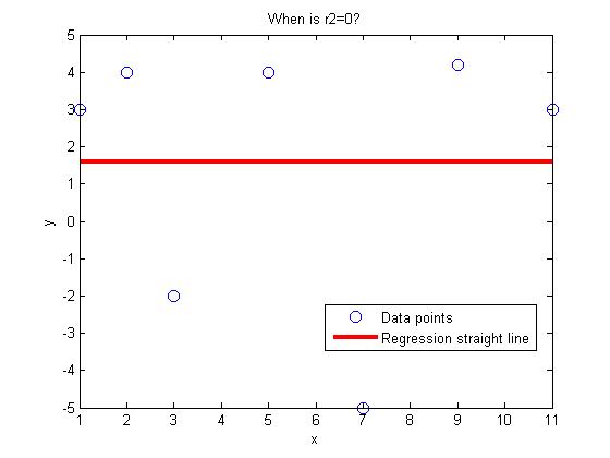
Do you choose based on the polynomial order for which the sum of the squares of the residuals, Sr is a minimum? If that were the case, we can always get Sr=0 if the polynomial order chosen is one less than the number of data points. In fact, it would be an exact match.

So what do we do? We choose the degree of polynomial for which the variance as computed by

Sr(m)/(n-m-1)

is a minimum or when there is no significant decrease in its value as the degree of polynomial is increased. In the above formula,

Sr(m) = sum of the square of the residuals for the mth order polynomial

n= number of data points

m=order of polynomial (so m+1 is the number of constants of the model)

Let’s look at an example where the coefficient of thermal expansion is given for a typical steel as a function of temperature. We want to relate the two using polynomial regression.

Temperature

Instantaneous Thermal Expansion

oF

1E-06 in/(in oF)

80

6.47

40

6.24

0

6.00

-40

5.72

-80

5.43

-120

5.09

-160

4.72

-200

4.30

-240

3.83

-280

3.33

-320

2.76

If a first order polynomial is chosen, we get

$latex alpha=0.009147T+5.999$, with Sr=0.3138.

If a second order polynomial is chosen, we get

$latex alpha=-0.00001189T^2+0.006292T+6.015$ with Sr=0.003047.

Below is the table for the order of polynomial, the Sr value and the variance value, Sr(m)/(n-m-1)

Order of

polynomial, m

Sr(m)

Sr(m)/(n-m-1)

1

0.3138

0.03486

2

0.003047

0.0003808

3

0.0001916

0.000027371

4

0.0001566

0.0000261

5

0.0001541

0.00003082

6

0.0001300

0.000325

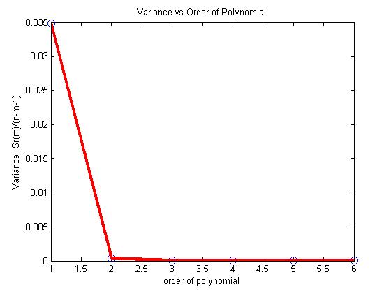
So what order of polynomial would you choose?

From the above table, and the figure below, it looks like the second or third order polynomial would be a good choice as very little change is taking place in the value of the variance after m=2.

Optimum order of polynomial for regression

This post is brought to you by Holistic Numerical Methods: Numerical Methods for the STEM undergraduate at http://nm.mathforcollege.com

Subscribe to the feed to stay updated and let the information follow you.

Data for aluminum cylinder in iced water experiment

A colleague asked me what if he did not have time or resources to do the experiments that have been developed at University of South Florida (USF) for numerical methods. He asked if I could share the data taken at USF.

Why not – here is the data for the experiment where an aluminum cylinder is placed in iced water. This link also has the exercises that the students were asked to do.

The temperature vs time data is as follows: (0,23.3), (5,16.3), (10,13), (15,11.8), (20,11), (25,10.7), (30,9.6), (35,8.9), (40,8.4). Time is in seconds and temperature in Celcius. Other data needed is

Ambient temperature of iced water = 1.1oC

Diameter of cylinder = 44.57 mm

Length of cylinder = 105.47 mm

Density of aluminum = 2700 kg/m3

Specific heat of aluminum = 901 J/(kg-oC)

Thermal conductivity of aluminum = 240 W/(m-K)

Table 1. Coefficient of thermal expansion vs. temperature for aluminum (Data taken from http://www.llnl.gov/tid/lof/documents/pdf/322526.pdf by using mid values of temperatures at which CTE is reported)

Temperature

(oC)

Coefficient of thermal expansion

(μm/m/oC)

-10

58

12.5

59

37.5

60

62.5

62

87.5

66

112.5

71

This post is brought to you by Holistic Numerical Methods: Numerical Methods for the STEM undergraduate at http://nm.mathforcollege.com

Subscribe to the feed to stay updated and let the information follow you.

In regression, when is coefficient of determination zero

The coefficient of determination is a measure of how much of the original uncertainty in the data is explained by the regression model.

The coefficient of determination, $latex r^2$ is defined as

$latex r^2$=$latex \frac{S_t-S_r}{S_r}$

where

$latex S_t$ = sum of the square of the differences between the y values and the average value of y

$latex S_r$ = sum of the square of the residuals, the residual being the difference between the observed and predicted values from the regression curve.

The coefficient of determination varies between 0 and 1. The value of the coefficient of determination of zero means that no benefit is gained by doing regression. When can that be?

One case comes to mind right away – what if you have only one data point. For example, if I have only one student in my class and the class average is 80, I know just from the average of the class that the student’s score is 80. By regressing student score to the number of hours studied or to his GPA or to his gender would not be of any benefit. In this case, the value of the coefficient of determination is zero.

What if we have more than one data point? Is it possible to get the coefficient of determination to be zero?

The answer is yes. Look at the following data pairs (1,3), (3,-2), (5,4), (7,-5), (9,4.2), (11,3), (2,4). If one regresses this data to a general straight line

y=a+bx,

one gets the regression line to be

y=1.6

When is rsquared zero?

In fact, 1.6 is the average value of the given y values. Is this a coincidence? Because the regression line is the average of the y values, $latex S_t=S_r$, implying $latex r^2=0$

QUESTIONS

  1. Given (1,3), (3,-2), (5,4), (7,a), (9,4.2), find the value of a that gives the coefficient of determination, $latex r^2=0$. Hint: Write the expression for $latex S_r$ for the regression line $latex y=mx+c$. We now have three unknowns, m, c and a. The three equations then are $latex \frac{\partial S_r} {\partial m} =0$, $latex \frac{\partial S_r} {\partial c} =0$ and $latex S_t=S_r$.
  2. Show that if n data pairs $latex (x_1,y_1)……(x_n,y_n)$ are regressed to a straight line, and the regression straight line turns out to be a constant line, then the equation of the constant line is always y=average value of the y-values.

This post is brought to you by Holistic Numerical Methods: Numerical Methods for the STEM undergraduate at http://nm.mathforcollege.com

Subscribe to the feed to stay updated and let the information follow you.