Integration – Page 2 – Numerical Methods Guy

How do I integrate a continuous function in MATLAB

Many students ask me how do I do this or that in MATLAB. So I thought why not have a small series of my next few blogs do that. In this blog I show you how to integrate a continuous function.

The MATLAB program link is here.

The HTML version of the MATLAB program is here.

___________________________________________

%% HOW DO I DO THAT IN MATLAB SERIES?
% In this series, I am answering questions that students have asked
% me about MATLAB. Most of the questions relate to a mathematical
% procedure.

%% TOPIC
% How do I integrate a continuous function?

%% SUMMARY

% Language : Matlab 2008a;
% Authors : Autar Kaw;
% Mfile available at
% http://nm.mathforcollege.com/blog/integration.m;
% Last Revised : March 28, 2009;
% Abstract: This program shows you how to integrate a given function.
clc
clear all

%% INTRODUCTION

disp(‘ABSTRACT’)
disp(‘   This program shows you how to integrate’)
disp(‘   a given function ‘)
disp(‘ ‘)
disp(‘AUTHOR’)
disp(‘   Autar K Kaw of http://autarkaw.wordpress.com’)
disp(‘ ‘)
disp(‘MFILE SOURCE’)
disp(‘   http://nm.mathforcollege.com/blog/integration.m’)
disp(‘ ‘)
disp(‘LAST REVISED’)
disp(‘   March 29, 2009’)
disp(‘ ‘)

%% INPUTS

% Integrate exp(x)*sin(3*x) from x=2.0 to 8.7
% Define x as a symbol
syms x
% Assigning the function to be differentiated
y=exp(x)*sin(3*x);
% Assigning the lower limit
a=2.0;
% Assigning the upper limit
b=8.7;

%% DISPLAYING INPUTS

disp(‘INPUTS’)
func=[‘ The function is to be integrated is ‘ char(y)];
disp(func)
fprintf(‘ Lower limit of integration, a= %g’,a)
fprintf(‘\n Upper limit of integration, b= %g’,b)
disp(‘ ‘)
disp(‘ ‘)

%% THE CODE

% Finding the integral using the int command
% Argument 1 is the function to be integrated
% Argument 2 is the variable with respect to which the
% function is to be integrated – the dummy variable
% Argument 3 is the lower limit of integration
% Argument 4 is the upper imit of integration
intvalue=int(y,x,a,b);
intvalue=double(intvalue);

%% DISPLAYING OUTPUTS

disp(‘OUTPUTS’)
fprintf(‘ Value of integral is = %g’,intvalue)
disp(‘ ‘)

_________________________________________________________

This post is brought to you by Holistic Numerical Methods: Numerical Methods for the STEM undergraduate at http://nm.mathforcollege.com, the textbook on Numerical Methods with Applications available from the lulu storefront, and the YouTube video lectures available at http://nm.mathforcollege.com/videos and http://www.youtube.com/numericalmethodsguy

Subscribe to the blog via a reader or email to stay updated with this blog. Let the information follow you.

MATLAB code for the efficient automatic integrator

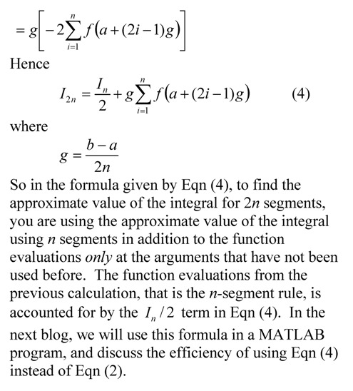
In the previous post, we discussed why doubling the number of segments in the automatic integrator based on multiple-segment trapezoidal rule is more efficient than increasing the number of segments one at a time. But this advantage involves having to store the individual function values from previous calculations and then having to retrieve them properly. This drawback was circumvented very efficiently by using the formula derived in another previous post where there is no need to store individual function values.

The matlab file for finding a definite integral by directly using the multiple segment trapezoidal rule from this post is given here (matlab file, html file), while the matlab file that uses the more efficient formula from this post is given here (matlab file, html file). Here are the inputs to the programs.

% a = Lower limit of integration
% b = Upper limit of integration
% nmax = Maximum number of segments
% tolerance = pre-specified tolerance in percentage
% f = inline function as integrand

a=5.3;
b=10.7;
nmax=200000;
tolerance=0.000005;
f=inline(‘exp(x)*sin(2*x)’)

We ran both the program on a PC and found that the more efficient algorithm (51 seconds) ran in half the time as the other one (82 seconds). This is expected, as only n function evaluations are made for 2n-segments rule with the efficient formula, while 2n+1 functions evaluations are made for the original formula.

Subscribe to the blog via a reader or email to stay updated with this blog. Let the information follow you.

An efficient formula for an automatic integrator based on trapezoidal rule

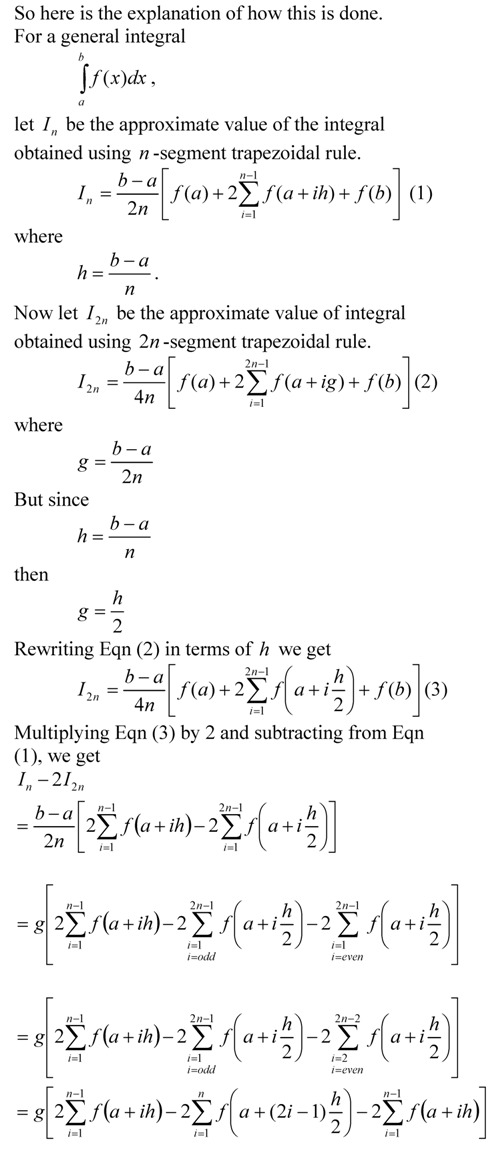
In the previous post, we discussed why doubling the number of segments in the automatic integrator based on multiple-segment trapezoidal rule is more efficient than increasing the number of segments one at a time. But this advantage involves having to store the individual function values from previous calculations and then having to retrieve them properly. This drawback can be circumvented very efficiently as explained below. What you will see is that there is no need to store individual function values.

Subscribe to the blog via a reader or email to stay updated with this blog. Let the information follow you.

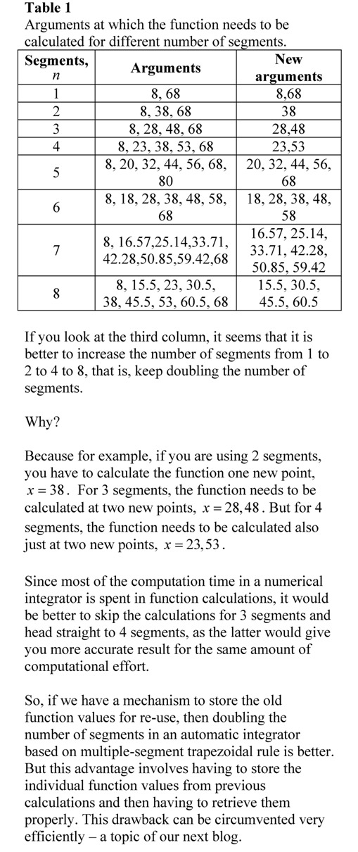
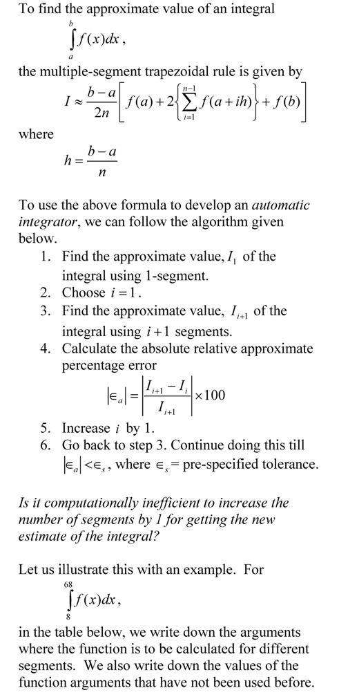
Why keep doubling the segments for an automatic integrator based on Trapezoidal rule?

Subscribe to the blog via a reader or email to stay updated with this blog. Let the information follow you.

An automatic integrator using Trapezoidal rule

How would you know how many segments to use in a Trapezoidal rule of integration to get an accurate value of the integral? This can be done by applying the Trapezoidal rule for 1 segment rule, then 2 segment rule, followed by 4 segment rule and so on. As soon as the absolute relative approximate error (page 5-6) between the consecutive answers becomes less than the pre-specified tolerance chosen by the user, you would have your integral within the accuracy you desired.

Here is a MATLAB program that does that for you. The MATLAB program that can be downloaded at http://nm.mathforcollege.com/blog/trapezoidal_rule_automatic.m (better to download it as single quotes from the web-post do not translate correctly with the MATLAB editor). The html file showing the mfile and the command window output is here: http://nm.mathforcollege.com/blog/html/trapezoidal_rule_automatic.html

% Simulation : Using Trapezoidal rule as an automatic integrator

% Language : Matlab 2007a

% Authors : Autar Kaw, http://nm.mathforcollege.com

% Mfile available at
% http://nm.mathforcollege.com/blog/trapezoidal_rule_automatic.m

% Last Revised : October 12, 2008

% Abstract: This program uses multiple-segment Trapezoidal
% rule to integrate f(x) from x=a to x=b within a pre-specified tolerance

clc
clear all

disp(‘This program uses multiple-segment Trapezoidal rule as an automatic integrator’)
disp(‘to integrate f(x) from x=a to x=b within a pre-specified tolerance’)
disp(‘ ‘)
disp(‘Author: Autar K Kaw.’)
disp(‘http://autarkaw.wordpress.com’)
disp(‘http://nm.mathforcollege.com’)
disp(‘ ‘)

%INPUTS. If you want to experiment, these are the only variables
% you should and can change.
% a = Lower limit of integration
% b = Upper limit of integration
% nmax = Maximum number of segments
% tolerance = pre-specified tolerance in percentage
% f = inline function as integrand
a=5.3;
b=10.7;
nmax=20000;
tolerance=0.005;
f=inline(‘exp(x)*sin(2*x)’);

% SIMULATION
disp(‘INPUTS’)
func=[‘     The integrand is =’ char(f)];
disp(func)
fprintf(‘     Lower limit of integration, a= %g’,a)
fprintf(‘\n     Upper limit of integration, b= %g’,b)
fprintf(‘\n     Maximum number of segments, nmax = %g’,nmax)
fprintf(‘\n     Pre-specified percentage tolerance, eps = %g’,tolerance)
disp(‘ ‘)
disp(‘ ‘)

% Doing the automatic integration
% Calculating the integral using 1-segment rule
previous_integral=(b-a)/2*(f(a)+f(b));
% Initializing ea as greater than pre-specified tolerance for loop to work
ea=2*tolerance;
% Starting with 2-segments inside the while loop
n=2;
while (ea>tolerance) & (n<=nmax)
h=(b-a)/n;
% Keeping track of used number of segments
nused=n;
current_integral=0;
for i=1:1:n-1
current_integral=current_integral+f(a+i*h);
end
current_integral=2*current_integral+f(a)+f(b);
current_integral=(b-a)/(2*n)*current_integral;
% Calculating the absolute relative approximate error
ea = abs((current_integral-previous_integral)/current_integral)*100;
previous_integral=current_integral;
% Doubling the number of segments for next estimate of the integral
n=n*2;
end

disp(‘OUTPUTS’)
fprintf(‘      Number of segments used =%g’, nused)
fprintf(‘\n      Approximate value of integral is =%g’,current_integral)
fprintf(‘\n      Absolute percentage relative approximate error =%g’, ea)
if (ea>tolerance)
disp(‘ ‘)
disp(‘ ‘)
disp(‘     NOTE: The value of integral is not within the pre-specified tolerance’)
end
disp(‘ ‘)

This post is brought to you by Holistic Numerical Methods: Numerical Methods for the STEM undergraduate at http://nm.mathforcollege.com.

An abridged (for low cost) book on Numerical Methods with Applications will be in print (includes problem sets, TOC, index) on December 10, 2008 and available at lulu storefront.

Subscribe to the blog via a reader or email to stay updated with this blog. Let the information follow you.

Another improper integral solved using trapezoidal rule

In a previous post, I showed how Trapezoidal rule can be used to solve improper integrals. The example used in the post was an improper integral with an infinite interval of integration.

In an example in this post, we use Trapezoidal rule to solve an improper integral where the integrand becomes infinite. The integral is $latex \int_{0}^{b} 1/sqrt{x} dx $. The integrand becomes infinite at x=0. Since x=0 would be one of the points where the integrand will be sought by the multiple-segment Trapezoidal rule, we choose the value of the integrand at x=0 to be zero (any other value would do too – a better assumption would be f(h), where h is the segment width in the multiple-segment Trapezoidal rule).

Here is a MATLAB program that shows you the exact value of the integral and then compares it with the multiple-segment Trapezoidal rule. The convergence is slow but you can integrate improper integrals using Trapezoidal rule.

The MATLAB program that can be downloaded at http://nm.mathforcollege.com/blog/trapezoidal_improper_sqrtx.m (better to download it as single quotes from the web-post do not translate correctly with the MATLAB editor). The html file showing the mfile and the command window output is here: http://nm.mathforcollege.com/blog/html/trapezoidal_improper_sqrtx.html

% Simulation : Can I use Trapezoidal rule for an improper integral?

% Language : Matlab 2007a

% Authors : Autar Kaw, http://nm.mathforcollege.com

% Mfile available at
% http://nm.mathforcollege.com/blog/trapezoidal_improper_sqrt.m

% Last Revised : October 8, 2008

% Abstract: This program shows use of multiple segment Trapezoidal
% rule to integrate 1/sqrt(x) from x=0 to b, b>0.

clc
clear all

disp(‘This program shows the convergence of getting the value of ‘)
disp(‘an improper integral using multiple segment Trapezoidal rule’)
disp(‘Author: Autar K Kaw. autarkaw.wordpress.com’)

%INPUTS. If you want to experiment, these are the only variables
% you should and can change.
% b = Upper limit of integration
% m = Maximum number of segments is 2^m
b=9;
m=14;

% SIMULATION
fprintf(‘\nFinding the integral of 1/sqrt(x) with limits of integration as x=0 to x=%g’,b)

% EXACT VALUE OF INTEGRAL
% integrand 1/sqrt(x)
syms x
f=1/sqrt(x);
a=0;
valexact=double(int(f,x,a,b));
fprintf(‘\n\nExact value of integral = %f’,valexact)
disp( ‘ ‘)

f=inline(‘1/sqrt(x)’);
%finding value of the integral using 16,…2^m segments
for k=4:1:m
n=2^k;
h=(b-a)/n;
sum=0;
for i=1:1:n-1
sum=sum+f(a+i*h);
end
% See below how f(a) is not added as f(a)=infinity. Instead we
% use a value of f(a)=0. How can we do that? Because as per integral calculus,
% using a different value of the function at one point or
% at finite number of points does not change the value of the
% integral.
sum=2*sum+0+f(b);
sum=(b-a)/(2*n)*sum;
fprintf(‘\nApproximate value of integral =%f with %g segments’,sum,n)
end
disp(‘ ‘)

This post is brought to you by Holistic Numerical Methods: Numerical Methods for the STEM undergraduate at http://nm.mathforcollege.com.

An abridged (for low cost) book on Numerical Methods with Applications will be in print (includes problem sets, TOC, index) on December 10, 2008 and available at lulu storefront.

Subscribe to the blog via a reader or email to stay updated with this blog. Let the information follow you.

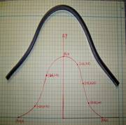
Experimental data for the length of curve experiment

In a previous post (click on the link on the left to learn fully about the experiment, and the assigned problems), I talked

about an experiment we conduct in class to compare spline and polynomial interpolation. If you do not want to conduct the experiment itself but want the (x,y) data to see for yourself how polynomial and spline interpolation compare, the data is given below.

Length of graduated flexible curve = 12″

The points on the x-y graph are as follows

(-4.1,0), (-2.6,1), (-2.0,2,2), (-1.6, 3.0), (-1,3.6), (0,3.9), (1.6,2.8), (3.2,0.4), (4.1,0)

________________________________________________________________________________________________

This post is brought to you by Holistic Numerical Methods: Numerical Methods for the STEM undergraduate at http://nm.mathforcollege.com.

An abridged (for low cost) book on Numerical Methods with Applications will be in print (includes problem sets, TOC, index) on December 10, 2008 and available at lulu storefront.

Subscribe to the blog via a reader or email to stay updated with this blog. Let the information follow you.

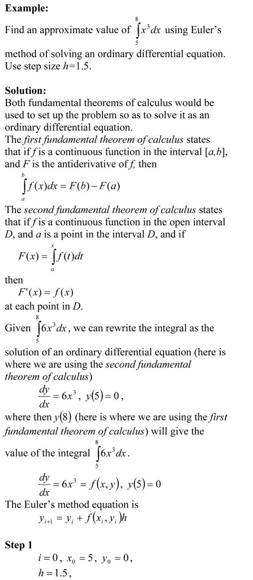
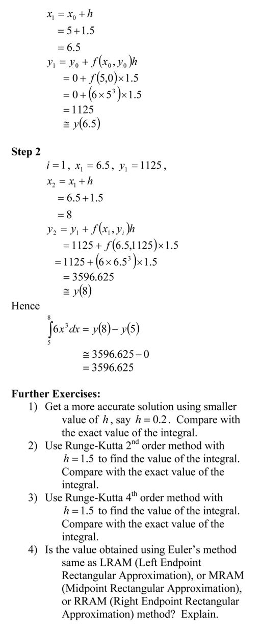
Example to show how numerical ODE solutions can be used to find integrals

In a previous post, I enumerated how we can use numerical ODE techniques like Euler and Runge-Kutta methods to find approximate value of definite integrals. Here is an example. Be sure to do the exercises at the end of the post to appreciate the procedure.

_____________________________________________________

This post is brought to you by Holistic Numerical Methods: Numerical Methods for the STEM undergraduate at http://nm.mathforcollege.com

Subscribe to the blog via a reader or email to stay updated with this blog. Let the information follow you.

Can I use numerical solution of ODE techniques to do numerical integration?

Yes.

If you are finding the value of the $latex y=\int_{a}^{b} f(x) dx$, then we can solve the integral as an ordinary differential equation as

dy/dx=f(x), y(a)=0

We can now use any of the numerical techniques such as Euler’s methods and Runge-Kutta methods to find the value of y(b) which would be the approximate value of the integral. Use exact techniques of solving linear ODEs with fixed coefficients such as Laplace transforms, and you can have the exact value of the integral.

_____________________________________________________

This post is brought to you by Holistic Numerical Methods: Numerical Methods for the STEM undergraduate at http://nm.mathforcollege.com

Subscribe to the blog via a reader or email to stay updated with this blog. Let the information follow you.

Is it just a coincidence – true error in multiple segment Trapezoidal rule gets approximately quartered as the number of segments is doubled?

Look at the table below. This is a table that shows the approximate value of the integral

$latex \int_{8}^{30} 2000 ln \frac{140000}{140000-2100t}-9.8t dt $

as a function of the number of segments used in the Trapezoidal rule and the corresponding true error.

n	Value	E_t
1	11868	-807
2	11266	-205
3	11153	-91.4
4	11113	-51.5
5	11094	-33.0
6	11084	-22.9
7	11078	-16.8
8	11074	-12.9

The true error for n=1 is -807 and for n=2 is -205. As you can see the quarter of -807 is approximately -201.75 and close to the true error for n=2. Is this a coincidence?

Look at the true error for n=2 which is -205 and for n=4 is -51.5. As you can see the quarter of -205 is approximately -51.75 and close to the value of the true error for n=4. Is this a coincidence?

No. This is because the true error in a single segment trapezoidal rule is

$latex \frac{(b-a)^3}{12} f^{\prime\prime} (c)$

where c is some point not known but in the domain [a,b] of $latex \int_{a}^{b} f(x) dx$. It can be then shown (see page 14 of this pdf file for full proof) that for the multiple segment trapezoidal rule, the true error is

$latex \frac{(b-a)^3}{12n^2} f^{\prime\prime} $

where the $latex f^{\prime\prime}$ is an average value of the second derivative of the function f(x) calculated at some point within each of the n segments. Since a and b are constant, and $latex f^{\prime\prime}$ becomes almost a constant as n increases, the true error is approximately inversely proportional to the square of the number of segments.

Note to the reader: Develop a similar table as given above for an integral of your choice and see it for yourself if the true error gets approximately quartered as the number of segments is doubled.

_____________________________________________________

This post is brought to you by Holistic Numerical Methods: Numerical Methods for the STEM undergraduate at http://nm.mathforcollege.com

Subscribe to the blog via a reader or email to stay updated with this blog. Let the information follow you.