Experiments for Numerical Methods – Numerical Methods Guy

Experimental data for the length of curve experiment

In a previous post (click on the link on the left to learn fully about the experiment, and the assigned problems), I talked

about an experiment we conduct in class to compare spline and polynomial interpolation. If you do not want to conduct the experiment itself but want the (x,y) data to see for yourself how polynomial and spline interpolation compare, the data is given below.

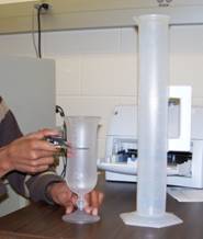
Length of graduated flexible curve = 12″

The points on the x-y graph are as follows

(-4.1,0), (-2.6,1), (-2.0,2,2), (-1.6, 3.0), (-1,3.6), (0,3.9), (1.6,2.8), (3.2,0.4), (4.1,0)

________________________________________________________________________________________________

This post is brought to you by Holistic Numerical Methods: Numerical Methods for the STEM undergraduate at http://nm.mathforcollege.com.

An abridged (for low cost) book on Numerical Methods with Applications will be in print (includes problem sets, TOC, index) on December 10, 2008 and available at lulu storefront.

Subscribe to the blog via a reader or email to stay updated with this blog. Let the information follow you.

Experiment for spline interpolation and integration

Background:

The motivation behind the experiment is to understand spline interpolation and numerical integration by finding the volume of water that can be held by a champagne glass.

What does the student do in the lab:

The student chooses one of the odd-shaped champagne glasses (Figure 1). The student measures the outer radius of the champagne glass at different known locations along the height. The student measures the thickness of the glass, so that he/she will be able to find the inner radius of the champagne glass at the locations he/she measured the outer radius. The student pours water to the brim in the champagne glass and checks how much volume the champagne glass holds.

Champagne Glass Exercises assigned to the students:
Use MATLAB to solve problems. Use comments, display commands and fprintf statements, sensible variable names and units to explain your work. Staple all the work in the following sequence. Use USCS system of units throughout.

Attach the data sheet on which you collected the data in class.
Find the spline interpolant that curve fits the radius vs height data.
Show the individual points and the spline interpolant of radius vs height on a single plot.
Find how much volume of water the champagne glass would hold.
Compare the above result from problem#4 to the actual volume.
In 100-200 words, type out your conclusions using a word processor. Any formulas should be shown using an equation editor. Any sketches need to be drawn using a drawing software such as Word Drawing. Any plots can be imported from MATLAB.

What materials do you need; where do I buy it; how much do the materials costs?

Champagne Glasses: These glasses, called the Hurricane Plastic Glasses, are available at www.poolsidepineapple.com, part nos. HUR-105, HUR-106, YAR-114. We used glasses made of plastic to avoid breakage. http:/www.poolsidepineapple.com/cart_pages/shopping%20page%20tropical.htm. You can try other places to buy the champagne glasses. About $40 or so for about six pieces including S&H. Better yet, go to a cruise and get souvenir glasses. Whenever you do the experiment, you will remember the good times.
Graduated Cylinder: The graduated cylinder is available at http://scientificsonline.com/, part number 3036286. The cost of the cylinder is $20+S&H.
Vernier Caliper: The caliper is available at http://mcmaster.com part number 20265A49. The cost of the vernier caliper is $60+S&H.
Scale: Need to buy a thin scale for this. Any art-supplies store for $2 or so.

_____________________________________________________

This post is brought to you by Holistic Numerical Methods: Numerical Methods for the STEM undergraduate at http://nm.mathforcollege.com

Subscribe to the blog via a reader or email to stay updated with this blog. Let the information follow you.

Length of a curve experiment

In a previous post, I mentioned that I have incorporated experiments in my Numerical Methods course. Here I will discuss the second experiment.

Length of the curve experiment In this experiment, we find the length of two curves generated from the same points – one curve is a polynomial interpolant and another one is a spline interpolant.

Motivation behind the experiment: In 1901, Runge conducted a numerical experiment to show that higher order interpolation is a bad idea. It was shown that as you use higher order interpolants to approximate f(x)=1/(1+25x²) in [-1,1], the differences between the original function and the interpolants becomes worse. This concept also becomes the basis why we use splines rather than polynomial interpolation to find smooth paths to travel through several discrete points.

What do students do in the lab: A flexible curve (see Figure) of length 12″ made of lead-core construction with graduations in both millimeters and inches is provided. The student needs to draw a curve similar in shape to the Runge’s curve on the provided graphing paper as shown. It just needs to be similar in shape – the student can make the x-domain shorter and the maximum y-value larger or vice-versa. The student just needs to make sure that there is a one-to-one correspondence of values.

Assigned Exercises: Use MATLAB to solve problems (3 thru 6). Use comments, display commands and fprintf statements, sensible variable names and units to explain your work. Staple all the work in the following sequence.

Signed typed affidavit sheet.
Attach the plot you drew in the class. Choose several points (at least nine – do not need to be symmetric) along the curve, including the end points. Write out the co-ordinates on the graphing paper curve as shown in the figure.
Find the polynomial interpolant that curve fits the data. Output the coefficients of the polynomial.
Find the cubic spline interpolant that curve fits the data. Just show the work in the mfile.
Illustrate and show the individual points, polynomial and cubic spline interpolants on a single plot.
Find the length of the two interpolants – the polynomial and the spline interpolant. Calculate the relative difference between the length of each interpolant and the actual length of the flexible curve.
In 100-200 words, type out your conclusions using a word processor. Any formulas should be shown using an equation editor. Any sketches need to be drawn using a drawing software such as Word Drawing. Any plots can be imported from MATLAB.

Where to buy the items for the experiment:

Flexible curves – I bought these via internet at Art City. The brand name is Alvin Tru-Flex Graduated Flexible Curves. Prices range from $5 to $12. Shipping and handling is extra – approximately $6 plus 6% of the price. You may want to buy several 12″ and 16″ flexible curves. I had to send a query to the vendor when I did not receive them within a couple of weeks. Alternatively, call your local Art Store and see if they have them.
Engineering Graph Paper – Staples or Office Depot. Costs about $12 for a pack for 100-sheet pad.
Pencil – Anywhere – My favorite store is the 24-hour Wal-Mart Superstore. $1 for a dozen.
Scale – Anywhere – My favorite store is the 24-hour Wal-Mart Superstore. $1 per unit.

This post is brought to you by Holistic Numerical Methods: Numerical Methods for the STEM undergraduate at http://nm.mathforcollege.com

Subscribe to the feed to stay updated and let the information follow you.

A legend used in the movie “The Happening”

Well M. Night Shyamalan may have made another disappointing movie – The Happening, but I somewhat liked it. I would give it a grade of B.

In the movie, John Leguzomo’s character, a math teacher, is distracting his fellow panicking passenger in the Jeep with a mathematical question. The question he asks her is if he gave her a penny on Day 1 of the month, two pennies on Day 2 of the month, four pennies on Day 3 of the month, and so on, how much would money would she have after a month. She shouts $300 or some odd number like that. But, do you know that the amount is actually more than a 10 million dollars (Thanks to a student who mentioned that it was a penny that John offered on the first day, not a dollar – sometimes I do feel generous).

This question is based on a story from India and it goes as follows.

King Shriham of India wanted to reward his grand minister Ben for inventing the game of chess. When asked what reward he wanted, Ben asked for 1 grain of rice on the first square of the board, 2 on the second square of the board, 4 on the third square of the board, 8 on the fourth square of the board, and so on till all the 64 squares were covered. That is, he was doubling the number of grains on each successive square of the board. Although Ben’s request looked less than modest, King Shriham quickly found that the amount of rice that Ben was asking for was humongous.

QUESTIONS:

Write a MATLAB (you can use any other programming language) program for the following using the for or while loop.

Find out how many grains of rice Ben was asking for.
If the mass of a grain of rice is 2 mg, and the world production of rice in recent years has been approximately 600,000,000 tons (1 ton=1000 kg), how many times the modern world production was Ben’s request?
Do the inverse problem – find out how many squares are covered if the the number of grains on the chess board are given to you. For example, how many squares will be covered if the number of grains on the chess board are 16?

This post is brought to you by Holistic Numerical Methods: Numerical Methods for the STEM undergraduate at http://nm.mathforcollege.com

Subscribe to the feed to stay updated and let the information follow you.

An experiment to illustrate numerical differentiation, integration, regression and ODEs

Aluminum Cylinder Dipped in Iced Water Starting Summer 2007, five experiments have been introduced in the course in Numerical Methods at USF. I will discuss each experiment in a separate blog as the

summer trods along.

Experiment#1: Cooling an aluminum cylinder

The first experiment illustrates use of numerical differentiation, numerical integration, regression and ordinary differential equations. In this experiment, an aluminum cylinder is immersed in a bath of iced water. As you can see in the figure, two thermocouples are attached to the cylinder and are connected to a temperature indicator. Readings of temperature as a function of time are taken in intervals of 5 seconds for a total of 40 seconds. The temperature of the iced-water bath is also noted.

If you just want the data for a typical experiment conducted in class, click here and here for data.

The students are now assigned about 10 problems to do. These include

finding the convection coefficient (involves nonlinear regression – it is also a good example of where the data for a nonlinear model does not need to be transformed to use linear regression)
finding the rate of change of temperature to calculate rate at which is heat is stored in the cylinder (involves numerical differentiation)
prediction of temperatures from solution of ordinary differential equations
finding reduction in the diameter of the aluminum cylinder (involves numerical integration as the thermal expansion coefficient is a function of temperature)

This post brought to you by Holistic Numerical Methods: Numerical Methods for the STEM undergraduate at http://nm.mathforcollege.com