One would intuitively assume that if one was given 100 data points of data, it would be most accurate to interpolate the 100 data points to a 99th order polynomial. More the merrier: is that not the motto. But I am sorry to burst your bubble – high order interpolation is generally a bad idea.
The classic example (dating as back as 1901 before there were calculators) to show that higher order interpolation idea is a bad idea comes from the famous German mathematician Carl Runge.
He took a simple and smooth function, f(x) = 1/(1+25x^2) in the domain [-1,1]. He chose equidisant x-data points on the function f(x) in the domain xε[-1,1]. Then he used those data points to draw a polynomial interpolant.
For example, if I chose 6 data points equidistantly spaced on [-1,1], those are (-1, 0.038462), (-0.6, 0.1), (-0.2,0.5), (0.2,0.5), (0.6,0.1), and (1,0.038462). I can interpolate these 6 data points by a 5th order polynomial. In Figure 1, I am then plotting the fifth order polynomial and the original function. You can observe that there is a large difference between the original function and the polynomial interpolant. The polynomial does go through the six points, but at many other points it does not even come close to the original function. Just look at x= 0.85, the value of the function is 0.052459, but the fifth order polynomial gives you a value of -0.055762, a whopping 206.30 % error; also note the opposite sign.
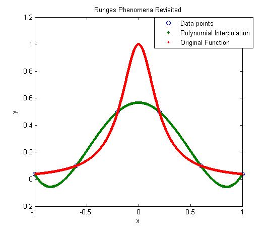
Figure 1. 5th order polynomial interpolation with six equidistant points.
Maybe I am not taking enough data points. Six points may be too small a number to approximate the function. Ok! Let’s get crazy. How about 20 points? That will give us a 19th order polynomial. I will choose 20 points equidistantly in [-1,1].
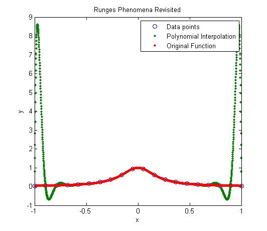
Figure 2. 19th order polynomial interpolation with twenty equidistant points
It is not any better though it did do a better job of approximating the function except near the ends. At the ends, it is worse than before. At our chosen point, x= 0.85, the value of the function is 0.052459, while we get -0.62944 from the 19th order polynomial, and that is a big whopper error of 1299.9 %.
So are you convinced that higher order interpolation is a bad idea? Try an example by yourself: step function y=-1, -1<x<0 and y=+1, 0<x<1.
What is the alternative to higher order interpolation? Is it lower order interpolation, but does that not use data only from less points than are given. How can we use lower order polynomials and at the same time use information from all the given data points. The answer to that question is SPLINE interpolation.
This post is brought to you by Holistic Numerical Methods: Numerical Methods for the STEM undergraduate at http://nm.mathforcollege.com
 Exercises assigned to the students:
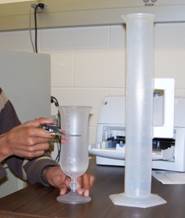
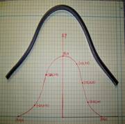 In this experiment, we find the length of two curves generated from the same points – one curve is a polynomial interpolant and another one is a spline interpolant.