runge – Numerical Methods Guy

Length of a curve experiment

In a previous post, I mentioned that I have incorporated experiments in my Numerical Methods course. Here I will discuss the second experiment.

Length of the curve experiment In this experiment, we find the length of two curves generated from the same points – one curve is a polynomial interpolant and another one is a spline interpolant.

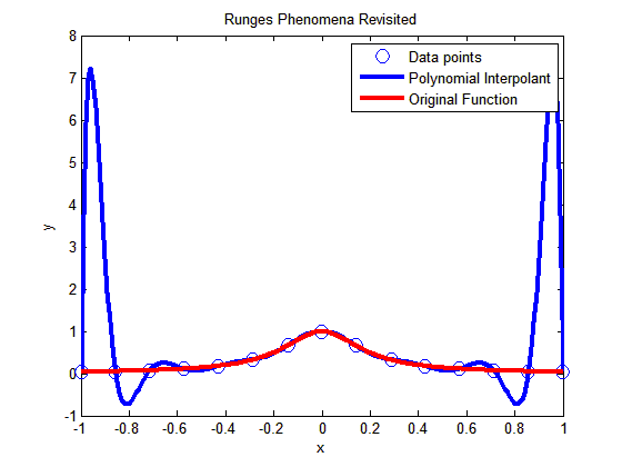
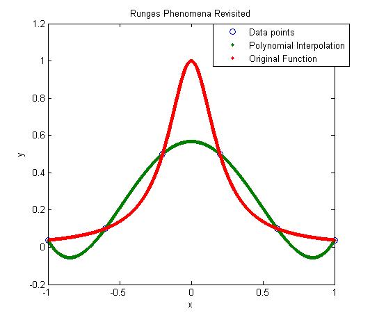
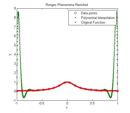
Motivation behind the experiment: In 1901, Runge conducted a numerical experiment to show that higher order interpolation is a bad idea. It was shown that as you use higher order interpolants to approximate f(x)=1/(1+25x²) in [-1,1], the differences between the original function and the interpolants becomes worse. This concept also becomes the basis why we use splines rather than polynomial interpolation to find smooth paths to travel through several discrete points.

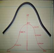
What do students do in the lab: A flexible curve (see Figure) of length 12″ made of lead-core construction with graduations in both millimeters and inches is provided. The student needs to draw a curve similar in shape to the Runge’s curve on the provided graphing paper as shown. It just needs to be similar in shape – the student can make the x-domain shorter and the maximum y-value larger or vice-versa. The student just needs to make sure that there is a one-to-one correspondence of values.

Assigned Exercises: Use MATLAB to solve problems (3 thru 6). Use comments, display commands and fprintf statements, sensible variable names and units to explain your work. Staple all the work in the following sequence.

Signed typed affidavit sheet.
Attach the plot you drew in the class. Choose several points (at least nine – do not need to be symmetric) along the curve, including the end points. Write out the co-ordinates on the graphing paper curve as shown in the figure.
Find the polynomial interpolant that curve fits the data. Output the coefficients of the polynomial.
Find the cubic spline interpolant that curve fits the data. Just show the work in the mfile.
Illustrate and show the individual points, polynomial and cubic spline interpolants on a single plot.
Find the length of the two interpolants – the polynomial and the spline interpolant. Calculate the relative difference between the length of each interpolant and the actual length of the flexible curve.
In 100-200 words, type out your conclusions using a word processor. Any formulas should be shown using an equation editor. Any sketches need to be drawn using a drawing software such as Word Drawing. Any plots can be imported from MATLAB.

Where to buy the items for the experiment:

Flexible curves – I bought these via internet at Art City. The brand name is Alvin Tru-Flex Graduated Flexible Curves. Prices range from $5 to $12. Shipping and handling is extra – approximately $6 plus 6% of the price. You may want to buy several 12″ and 16″ flexible curves. I had to send a query to the vendor when I did not receive them within a couple of weeks. Alternatively, call your local Art Store and see if they have them.
Engineering Graph Paper – Staples or Office Depot. Costs about $12 for a pack for 100-sheet pad.
Pencil – Anywhere – My favorite store is the 24-hour Wal-Mart Superstore. $1 for a dozen.
Scale – Anywhere – My favorite store is the 24-hour Wal-Mart Superstore. $1 per unit.

This post is brought to you by Holistic Numerical Methods: Numerical Methods for the STEM undergraduate at http://nm.mathforcollege.com

Subscribe to the feed to stay updated and let the information follow you.

A simple MATLAB program to show that High order interpolation is a bad idea

In a previous post, we talked about that higher order interpolation is a bad idea.

Runge's function

In this post I am showing you a MATLAB program that will allow you to experiment by changing the number of data points you choose, that is, the value of n (see the input highlighted in red in the code – this is the only line you want to change) and see for yourself why high order interpolation is a bad idea. Just, cut and paste the code below (or download it from http://www.eng.usf.edu/~kaw/download/runge.m) in the MATLAB editor and run it.

% Simulation : Higher Order Interpolation is a Bad Idea

% Language : Matlab r12
% Authors : Autar Kaw
% Last Revised : June 10 2008
% Abstract: In 1901, Carl Runge published his work on dangers of high order
% interpolation. He took a simple looking function f(x)=1/(1+25x^2) on
% the interval [-1,1]. He took points equidistantly spaced in [-1,1]
% and interpolated the points with polynomials. He found that as he
% took more points, the polynomials and the original curve differed
% even more considerably. Try n=5 and n=25
clc
clear all
clf

disp(‘In 1901, Carl Runge published his work on dangers of high order’)
disp(‘interpolation. He took a simple looking function f(x)=1/(1+25x^2) on’)
disp(‘the interval [-1,1]. He took points equidistantly spaced in [-1,1]’)
disp(‘and interpolated the points with a polynomial. He found that as he’)
disp(‘took more points, the polynomials and the original curve differed’)
disp(‘even more considerably. Try n=5 and n=15’)

%
% INPUT:
% Enter the following
% n= number of equidisant x points from -1 to +1
n=15;

% SOLUTION
disp(‘ ‘)
disp(‘SOLUTION’)
disp(‘Check out the plots to appreciate: High order interpolation is a bad idea’)
fprintf(‘\nNumber of data points used =%g’,n)
% h = equidisant spacing between points
h=2.0/(n-1);
syms xx
% generating n data points equally spaced along the x-axis
% First data point
x(1)=-1;
y(1)=subs(1/(1+25*xx^2),xx,-1);
% Other data points
for i=2:1:n
x(i)=x(i-1)+h;
y(i)=subs(1/(1+25*xx^2),xx,x(i));
end

% Generating the (n-1)th order polynomial from the n data points
p=polyfit(x,y,n-1);

% Generating the points on the polynomial for plotting
xpoly=-1:0.01:1;
ypoly=polyval(p,xpoly);

% Generating the points on the function itself for plotting
xfun=-1:0.01:1;
yfun=subs(1/(1+25*xx^2),xx,xfun);

% The classic plot
% Plotting the points
plot(x,y,’o’,’MarkerSize’,10)
hold on
% Plotting the polynomial curve
plot(xpoly,ypoly,’LineWidth’,3,’Color’,’Blue’)
hold on
% Plotting the origianl function
plot(xfun,yfun,’LineWidth’,3,’Color’,’Red’)
hold off
xlabel(‘x’)
ylabel(‘y’)
title(‘Runges Phenomena Revisited’)
legend(‘Data points’,’Polynomial Interpolant’,’Original Function’)
%***********************************************************************
disp(‘ ‘)
disp(‘ ‘)
disp(‘What you will find is that the polynomials diverge for’)
disp(‘0.726<|x|<1. If you started to choose same number of points ‘)
disp(‘but more of them close to -1 and +1, you would avoid such divergence. ‘)
disp(‘ ‘)
disp(‘However, there is no general rule to pick points for a general ‘)
disp(‘function so that this divergence is avoided; but some rules do exist for ‘)
disp(‘certian types of functions.’)

This post is brought to you by Holistic Numerical Methods: Numerical Methods for the STEM undergraduate at http://nm.mathforcollege.com

High order interpolation is a bad idea?

One would intuitively assume that if one was given 100 data points of data, it would be most accurate to interpolate the 100 data points to a 99th order polynomial. More the merrier: is that not the motto. But I am sorry to burst your bubble – high order interpolation is generally a bad idea.

The classic example (dating as back as 1901 before there were calculators) to show that higher order interpolation idea is a bad idea comes from the famous German mathematician Carl Runge.

He took a simple and smooth function, f(x) = 1/(1+25x^2) in the domain [-1,1]. He chose equidisant x-data points on the function f(x) in the domain xε[-1,1]. Then he used those data points to draw a polynomial interpolant.

For example, if I chose 6 data points equidistantly spaced on [-1,1], those are (-1, 0.038462), (-0.6, 0.1), (-0.2,0.5), (0.2,0.5), (0.6,0.1), and (1,0.038462). I can interpolate these 6 data points by a 5th order polynomial. In Figure 1, I am then plotting the fifth order polynomial and the original function. You can observe that there is a large difference between the original function and the polynomial interpolant. The polynomial does go through the six points, but at many other points it does not even come close to the original function. Just look at x= 0.85, the value of the function is 0.052459, but the fifth order polynomial gives you a value of -0.055762, a whopping 206.30 % error; also note the opposite sign.

Figure 1. 5th order polynomial interpolation with six equidistant points.

Maybe I am not taking enough data points. Six points may be too small a number to approximate the function. Ok! Let’s get crazy. How about 20 points? That will give us a 19th order polynomial. I will choose 20 points equidistantly in [-1,1].

Figure 2. 19th order polynomial interpolation with twenty equidistant points

It is not any better though it did do a better job of approximating the function except near the ends. At the ends, it is worse than before. At our chosen point, x= 0.85, the value of the function is 0.052459, while we get -0.62944 from the 19th order polynomial, and that is a big whopper error of 1299.9 %.

So are you convinced that higher order interpolation is a bad idea? Try an example by yourself: step function y=-1, -1<x<0 and y=+1, 0<x<1.

What is the alternative to higher order interpolation? Is it lower order interpolation, but does that not use data only from less points than are given. How can we use lower order polynomials and at the same time use information from all the given data points. The answer to that question is SPLINE interpolation.

This post is brought to you by Holistic Numerical Methods: Numerical Methods for the STEM undergraduate at http://nm.mathforcollege.com