Why I do not allow cell phones or regular laptops in class

I do not allow cell phones and regular laptops in my class – it is considered academic disruption. If someone is expecting an important call, I ask them to let me know and sit in chairs close to the classroom exit door. Very few people take me on that offer over a semester even in a class of 109. “Loved ones including mine should call 911 in case of an emergency – the emergency response team will be there faster than we can.”

I do allow flat laptops and tablets only if they are used to take notes with a stylus. They cannot claim that they want to type notes as that is virtually impossible to do in an engineering course full of equations and sketches. Anyway, taking notes by hand is cognitively better than typing anyway.

About those of you who keep mentioning personal responsibility and that it is an ego trip for the instructor, how many studies do I need to show you about negative effects of multitasking and working memory when one is learning something new.

About personal responsibility, it is more than that – the cell phone distracts others and there are studies on that too.  And removing temptation is much better than self-control.

About those who say, be more interesting than the incoming text – I cannot compete, as learning something new is hard and looking at a “Facebook like” is an immediate high. My lecture is anticipated if I am doing a good job of constructing knowledge but a text is a Pavlov’s bell.

_____________________________________________________

This post is brought to you by

Background Example for Newton Raphson Method

One of the three tenets of a student succeeding in a course is how well he knows the pre-requisite knowledge for the course (other two tenets are ability and interest).  We as instructors can make it easier for students to get to a reasonable competency level by offering short reviews of the pre-requisite knowledge in form of video and/or text.

Here , a student will review via an example the background needed to learn Newton-Raphson method of solving a nonlinear equation of the form f(x)=0.

For more videos and resources on this topic, please visit http://nm.mathforcollege.com/topics/newton_raphson.html

________________________

This post is brought to you by

Research Grant Offered to Improve Flipped Classroom through Adaptive Learning

Dr. Autar Kaw receives a grant to lead improvement of flipped classrooms through adaptive learning

Tampa, FL (December 20, 2016) – Ever since Autar Kaw started teaching at the University of South Florida in 1987, he has used evidence-based pedagogies such as interactive instructional software and active learning in the classroom.  Since 2001, he has been conducting federally funded research in transforming undergraduate engineering education through development and assessment of open resources for undergraduate courses such as Numerical Methods.

With his success of using blended learning for more than a decade and having been the lead developer of a comprehensive open courseware for Numerical Methods, the National Science Foundation (NSF) granted a four-institution (University of South Florida, Arizona State University, Alabama A&M, and University of Pittsburgh) grant in 2013 to determine the effectiveness of flipped learning classroom.  As per the Flipped Learning Network, “Flipped Learning is a pedagogical approach in which direct instruction moves from the group learning space to the individual learning space, and the resulting group space is transformed into a dynamic, interactive learning environment where the educator guides students as they apply concepts and engage creatively in the subject matter.”  The research from the grant indicated positive improvement in student learning gains through flipped learning but challenges persisted in some students coming inadequately prepared for the classroom meeting.  Although before class they were required to study through their preference of video lectures or textbook, and take an automatically-graded online quiz, it still was a single recipe prescribed for all.

To address this concern of pre-class preparation, NSF has given Professor Kaw and his colleague Professor Mary Besterfield-Sacre of University of Pittsburgh an Engaged Student Learning Exploration and Design grant that will use the adaptive platform of Knewton, Inc to personalize the pre-class activities for every learner.  Knewton’s mission is to support and challenge every student to meet their learning goals through personalized learning.

flippedclassroomuwcolorsTraditional vs Flipped Classroom (Photo Courtesy of University of Washington – Center for Teaching and Learning and Office of the Provost)

To improve the pre-class activities of the flipped class, the instructional and assessment modules from prior NSF support are being augmented and revised to conform to the Knewton adaptive platform. Specifically, the project will be comparing the effectiveness of three instructional approaches: a flipped class with adaptive learning, a flipped class without adaptive learning, and a blended class without adaptive learning, based on student conceptual gains, procedural knowledge, higher-order problem solving, and affective learning. These comparisons will be conducted statistically at a granular level using the factors of GPA, gender, race, age, transfer status, socioeconomic status, working hours, course topic, proficiency levels, and time on task, as well as qualitatively via focus groups and interviews.  This work will hence advance the understanding of the impact of the combined flipped and adaptive approaches on cognitive and affective learning gains of students representing diverse populations.

This project will specifically provide materials and best practices for teaching Numerical Methods in a flipped setting on an adaptive platform and provide new viable opportunities to how STEM courses are taught. This effort will also take us closer to meeting the NAE’s 21st Century Grand Challenge of “Advance Personalized Learning”.  Dissemination avenues include the freely-available Knewton adaptive platform, an open education resource portal from prior support, and social media.

For more information about the project, send an email to kaw@usf.edu.

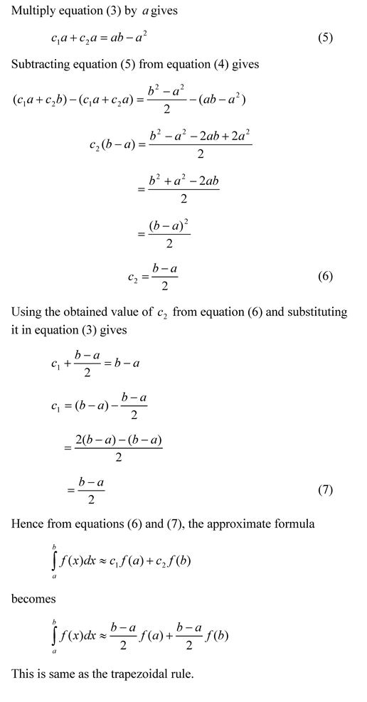
Deriving trapezoidal rule using undetermined coefficients

trapezoidal-coefficients_page_1trapezoidal-coefficients_page_2

_______________________________________

This post is brought to you by

Implications of diagonally dominant matrices

In the previous blogs (Part 1, Part 2, Part 3, Part 4), we clarified the difference and similarities between diagonally dominant matrices, weakly diagonal dominant matrices, strongly diagonally dominant matrices, and irreducibly diagonally dominant matrices.  In this blog, we enumerate what implications these classifications have.

_____________________________

If a square matrix is strictly diagonally dominant

  • then the matrix is non-singular [1].
  • then if the matrix is symmetric with non-negative diagonal entries, the matrix is positive semi-definite [1].
  • then if the matrix is the coefficient matrix for a set of simultaneous linear equations, the iterative Gauss-Seidel numerical method will always converge [2].
  • then if the matrix is the coefficient matrix for a set of simultaneous linear equations, the iterative Jordan numerical method will always converge [2].
  • then if the diagonal entries of the matrix are positive, the real parts of the matrix eigenvalues are positive [1].
  • then if the diagonal entries of the matrix are negative, the real parts of the matrix eigenvalues are negative [1].
  • then if the matrix is column dominant, no pivoting is needed for Gaussian elimination [2].
  • then if the matrix is column dominant, no pivoting is needed for LU factorization [2].

_______________________________

If a square matrix is irreducible diagonally dominant

  1. then if the matrix is the coefficient matrix for a set of simultaneous linear equations, the iterative Gauss-Seidel numerical method will always converge.
  2. then if the matrix is the coefficient matrix for a set of simultaneous linear equations, the iterative Jordan numerical method will always converge.
  3. the matrix is non-singular [2].

________________________________

If a square matrix is diagonally dominant (also called weakly diagonally dominant)

  1. then if the matrix is column dominant, no pivoting is needed for Gaussian elimination [3].
  2. then if the matrix is column dominant, no pivoting is needed for LU factorization [3].

References

  1. Briggs, Keith. “Diagonally Dominant Matrix.” FromMathWorld–A Wolfram Web Resource, created by Eric W. Weisstein.  http://mathworld.wolfram.com/DiagonallyDominantMatrix.html
  1. Diagonally Dominant Matrix, see https://en.wikipedia.org/wiki/Diagonally_dominant_matrix, Last accessed on November 4, 2016.
  1. “Lecture 4: A Gaussian Elimination Example”, see http://www.cs.yale.edu/homes/spielman/BAP/lect4.pdf, last accessed on November 4, 2016.

_______________________________________

This post is brought to you by

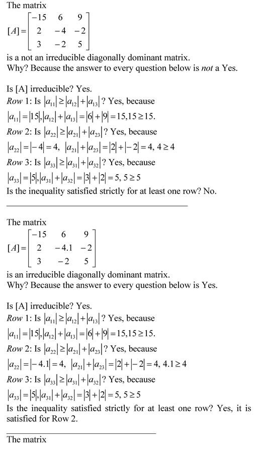
Clearing up the confusion about diagonally dominant matrices – Part 4

irreducible_diagonally_dominant1_page_1irreducible_diagonally_dominant1_page_2irreducible_diagonally_dominant1_page_3
You can view the above document as a pdf file as well.

Other blogs on diagonally dominant matrices
Clearing up the confusion about diagonally dominant matrices – Part 1

Clearing up the confusion about diagonally dominant matrices – Part 2

Clearing up the confusion about diagonally dominant matrices – Part 3

_________________________________________________________

This post is brought to you by

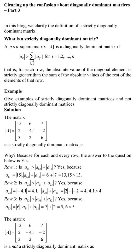
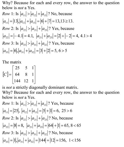
Clearing up the confusion about diagonally dominant matrices – Part 3

You can view the above document as a pdf file as well.

Other blogs on diagonally dominant matrices
Clearing up the confusion about diagonally dominant matrices – Part 1

Clearing up the confusion about diagonally dominant matrices – Part 2

_________________________________________________________

This post is brought to you by

Clearing up the confusion about diagonally dominant matrices – Part 2

In a previous post, we discussed the confusion about the definition and associated properties of diagonally dominant matrices.  In this blog, we answer the next question.

What is a weak diagonally dominant matrix?

The answer is simple – the definition of a weak(ly) diagonally dominant matrix is identical to that of a diagonally dominant matrix as the inequality used for the check is a weak inequality of greater than or equal to (≥).  See the previous post on Clearing up the confusion about diagonally dominant matrices – Part 1 where we define a diagonally dominant matrix.

Other blogs on diagonally dominant matrices
Clearing up the confusion about diagonally dominant matrices – Part 1

_______________________________________

This post is brought to you by


Clearing up the confusion about diagonally dominant matrices – Part 1

You can view the above document as a pdf file as well.

_________________________________________________________

This post is brought to you by

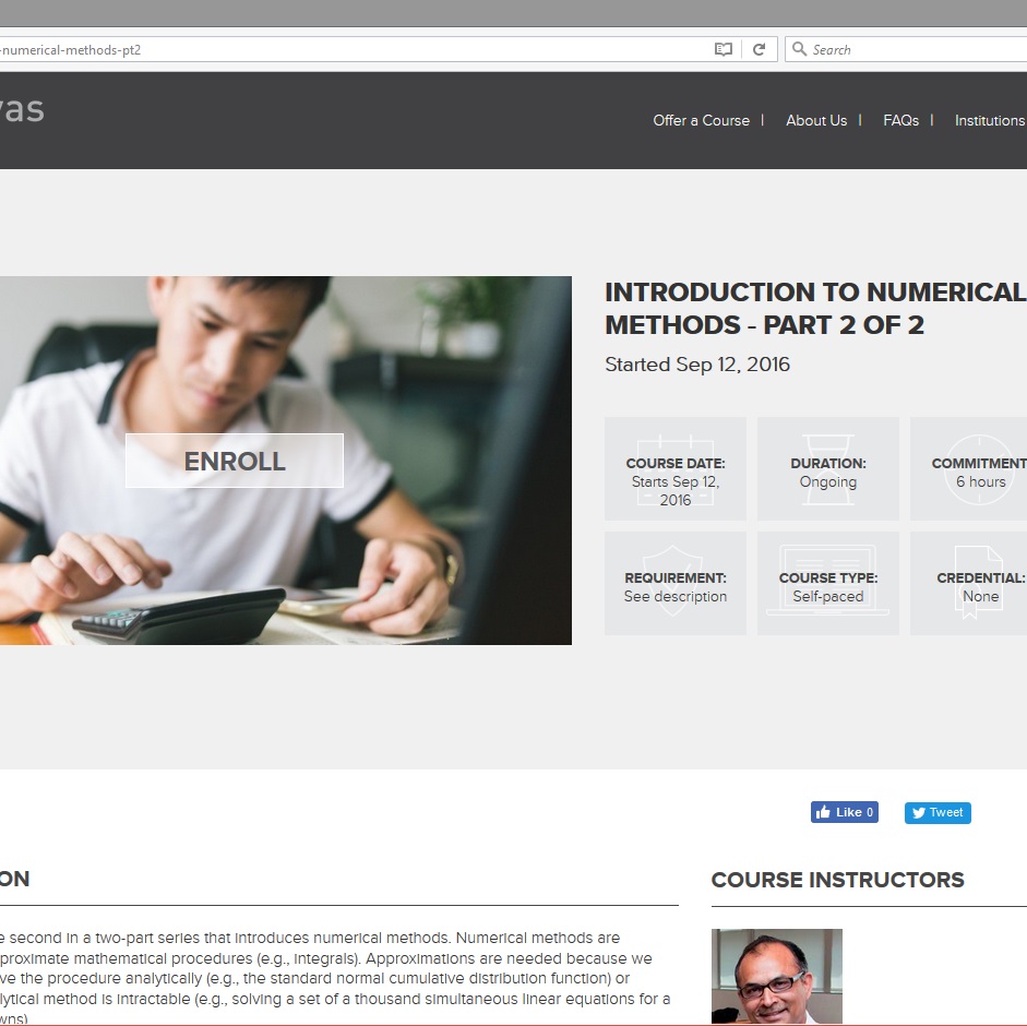
MOOC Released:Introduction to Numerical Methods – Part 2 of 2

After the rigorous and comprehensive development and assessment of the NSF-funded innovative open courseware on Numerical Methods since 2002, we are offering a FREE Massive Open Online Course (MOOC) in Numerical Methods – Part 2 of 2 at https://learn.canvas.net/courses/1189

This part of the MOOC covers the mathematical procedures of interpolation, regression, integration and ordinary differential equations.

The Part 1 of 2 of the course is also available and is at https://learn.canvas.net/courses/1065

Start your journey today whether you are learning numerical methods for the first time or just need a refresher.  Unlike other MOOCs, you have a lifetime (mine) access to the course and you can pace yourself. Ask questions within the course and we will keep the conversation going!

part2of2

About: Numerical methods are techniques to approximate mathematical procedures (an example of a mathematical procedure is an integral).  Approximations are needed because we either cannot solve the procedure analytically (an example is the standard normal cumulative  distribution function) or because the analytical method is intractable (an example is solving a set of a thousand simultaneous linear equations for a thousand unknowns).

Materials Included: Textbook Chapters, Video Lectures, Quizzes, Solutions to Quizzes

How Long to Complete: About 20 hours of lectures need to be watched and estimated  time to read the textbook and do quizzes is 40 hours.  It is a typical 7-week semester length course.

Course Structure: For each section, you have video lectures, followed by a textbook chapter, a quiz and its complete solution, and automatically graded online quizzes.

____________________________________________________________

This post is brought to you by