An experiment to illustrate numerical differentiation, integration, regression and ODEs

Aluminum Cylinder Dipped in Iced WaterStarting Summer 2007, five experiments have been introduced in the course in Numerical Methods at USF. I will discuss each experiment in a separate blog as the

summer trods along.

Experiment#1: Cooling an aluminum cylinder

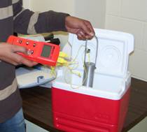
The first experiment illustrates use of numerical differentiation, numerical integration, regression and ordinary differential equations. In this experiment, an aluminum cylinder is immersed in a bath of iced water. As you can see in the figure, two thermocouples are attached to the cylinder and are connected to a temperature indicator. Readings of temperature as a function of time are taken in intervals of 5 seconds for a total of 40 seconds. The temperature of the iced-water bath is also noted.

If you just want the data for a typical experiment conducted in class, click here and here for data.

The students are now assigned about 10 problems to do. These include

  1. finding the convection coefficient (involves nonlinear regression – it is also a good example of where the data for a nonlinear model does not need to be transformed to use linear regression)
  2. finding the rate of change of temperature to calculate rate at which is heat is stored in the cylinder (involves numerical differentiation)
  3. prediction of temperatures from solution of ordinary differential equations
  4. finding reduction in the diameter of the aluminum cylinder (involves numerical integration as the thermal expansion coefficient is a function of temperature)

This post brought to you by Holistic Numerical Methods: Numerical Methods for the STEM undergraduate at http://nm.mathforcollege.com

Rusty on Matrix Algebra

Eight years ago, the Florida legislature decided to reduce the number of credit hours it takes a state university student to graduate with an undergrad engineering degree. The number of credit hours were reduced from 136 to 128. One of the courses that got the ax in the Mechanical Engineering Department at USF was a 2-credit hour Linear Algebra course. There are many other universities in the nation that have done the same.

So how do students learn Linear Algebra when the course is one of the requirements for accreditation of engineering programs?

Some universities have bundled Linear Algebra course content into courses such as Quantitative Methods where students are expected, in many cases, to learn linear algebra, a programming language/computational system, and complex analysis. Other curriculums have dispersed the Linear Algebra content into different courses such as the topic of special matrices in Programming, simultaneous linear equations in Statics, and eigenvalues/eigenvectors in Vibrations, etc. Unless quality controls are introduced carefully, the content/depth of Linear Algbera in such courses can vary substantially between courses and instructors. Such control is impossible in metropolitan universities such as USF where a large proportion of students transfer from community colleges.

To have a resource that would be a self-explanatory as well as get the students exposed to Linear Algebra applications motivated me to write a simple Introduction to Matrix Algebra book. The book consists of ten chapters spanning fundamentals of matrix algebra, numerical methods for solving a set of equations, and a treatment of adequacy of solutions and eigenvalues.

Since 2002, the Introduction to Matrix Algebra book has been downloaded free of charge by more than 30,000 users from 50 different countries, and the feedback has been humbling and fulfilling.

Since April 2008, the book has also been made available for a nominal charge via lulu.com as a pdf file as well as a soft cover book. Proceeds from the book are allowing me to expand the book with more examples/problems and additional chapters.

Since my belief continues to embrace open and uncomplicated dissemination, eight individual chapters of the book in pdf form are still available free of charge. So one may ask the following question. Why should I buy the book when it is available free of charge? For answer to this question, click here

For more details about the book, visit the book website at http://autarkaw.com/books/matrixalgebra/index.html

This post brought to you by Holistic Numerical Methods: Numerical Methods for the STEM undergraduate at http://nm.mathforcollege.com

LU Decomposition takes more computational time than Gaussian Elimination! What gives?

If you are solving a set of simultaneous linear equations, LU Decomposition method (involving forward elimination, forward substitution and back substitution) would use more computational time than Gaussian elimination (involving forward elimination and back substitution, but NO forward substitution).

So why use and waste time talking about LU Decomposition?

Because, LU Decomposition is computationally more efficient than Gaussian elimination when we are solving several sets of equations with the same coefficient matrix but different right hand sides. Case in point is when you are finding the inverse of a matrix [A]. If one is trying to find the inverse of nxn matrix, then it implies that one needs to solve n sets of simultaneous linear equations of [A][X]=[C] form with the n right hand sides [C] being the n columns of the nxn identity matrix, while the coefficient matrix [A] stays the same.

The computational time taken for solving a single set of n simultaneous linear equations is as follows:

  • Forward elimination: Proportional to \frac{n^3}{3}
  • Back substitution: Proportional to \frac{n^2}{2}
  • Forward substitution: Proportional to \frac{n^2}{2}

So for LU decomposition method used to find the inverse of a matrix, the computational time is proportional to \frac{n^3}{3}+n( \frac{n^2}{2}+\frac{n^2}{2})=\frac{4n^3}{3}. Remember that the forward elimination only needs to be done only once on [A] to generate the L and U matrices for the LU decomposition method. However the forward and back substitution need to be done n times.

Now for Gaussian Elimination used to find the inverse of a matrix, the computational time is proportional to n \frac{n^3}{3} +n \frac{n^2}{2}=\frac{n^4}{3}+\frac{n^3}{2}. Remember that both the forward elimination and back substitution need to be done n times.

Hence for large n, for LU Decomposition, the computational time is proportional to \frac{4n^3}{3}, while for Gaussian Elimination, the computational time is proportional to \frac{n^4}{3} . So for large n, the ratio of the computational time for Gaussian elimination to computational for LU Decomposition is {\frac{n^4}{3}}/{\frac{4n^3}{3}}=\frac{n}{4}

As an example, to find the inverse of a 2000×2000 coefficient matrix by Gaussian Elimination would take n/4=2000/4=500 times the time it would take to find the inverse by LU Decomposition.

So are you convinced now why we use LU Decomposition in certain cases? For textbook notes on this issue, examples of LU Decomposition to solve a set of equations, and finding inverse of a matrix using LU Decomposition, click here.

Reference: Numerical Methods for the STEM Undergraduate, http://nm.mathforcollege.com/topics/lu_decomposition.html

This post brought to you by Holistic Numerical Methods: Numerical Methods for the STEM undergraduate at http://nm.mathforcollege.com

Undergraduate Numerical Methods for Engineering

I am starting this blog to help UNDERGRADUATES with their queries on Numerical Methods for Engineers. I have been teaching Numerical Methods for the last 20 years and I get interesting queries and questions while I am teaching, when students come to see me during my office hours, or the email sent at midnight before the assignment is due.

I am keeping a log of what students ask me and will note the answers to their queries here. I am sure that students elsewhere have similar questions when they take a course in Numerical Methods.

The diversity of the course is quite evident –

  1. The course is taught to different engineering majors – mechanical, civil, chemical, industrial and electrical.
  2. Some teachers emphasize the numerical methods while others spend more time on solving physical problems, and a few may include numerical analysis.
  3. The programming tools are diverse including FORTRAN (yes the language is alive and well), Basic, C, Java, or computational packages such as MATLAB, MATHEMATICA, MathCAD, and Maple.

With funding from NSF since 2002, we have developed web-based resources for a course in Numerical Methods. The inclusion of the blog is not part of the funded proposals but we think that this mode of Web 2.0 dissemination is critical in keeping the conversation going on. Although what I am doing here can be offered via a static website, the widgets offered by blogging softwares are indispensable. The widgets I like are categorizing, tagging and RSS Feeds.

We want to reach as many people as possible and build a community which may be temporary to students who are taking a course in Numerical Methods, permanent to instructors and people who use numerical methods in their work. But one thing is certain, temporary or permanent, visitors will leave their imprint on this resource.

This post brought to you by Holistic Numerical Methods: Numerical Methods for the STEM undergraduate at http://nm.mathforcollege.com