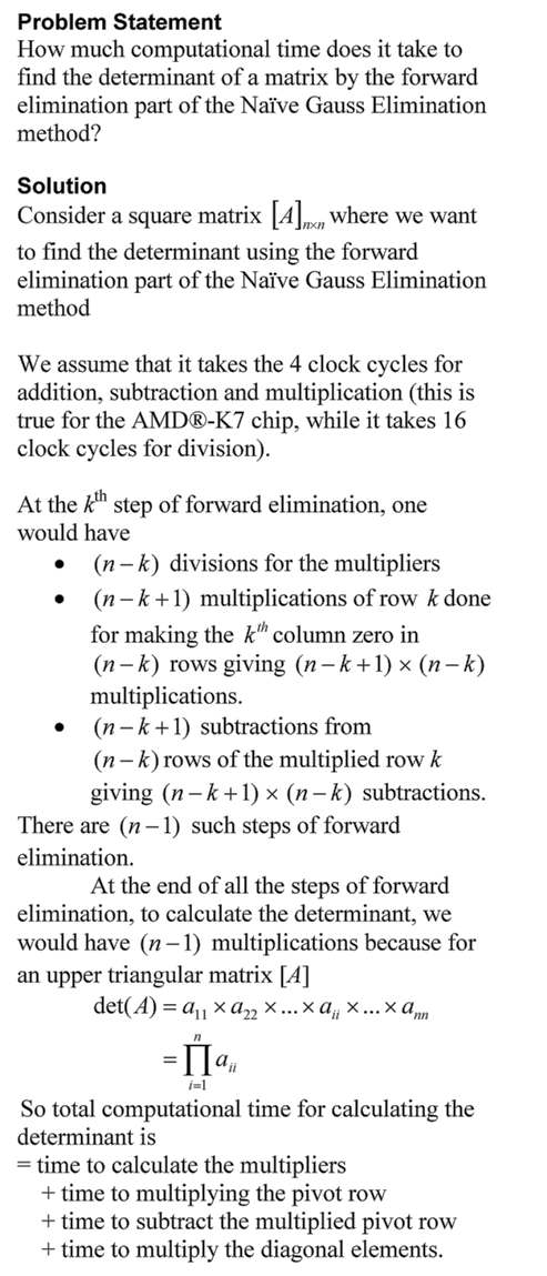
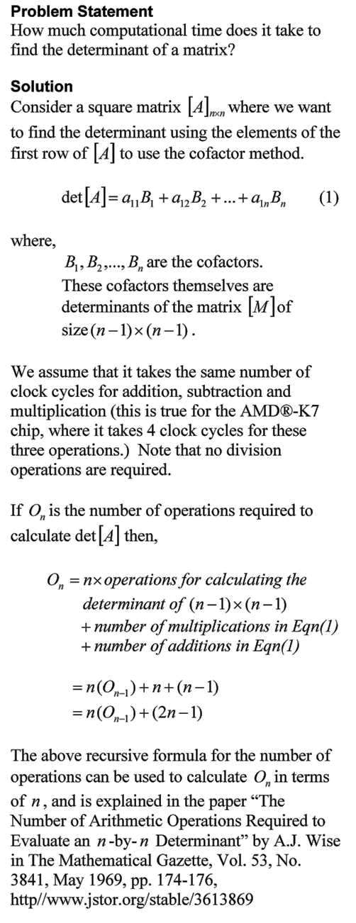
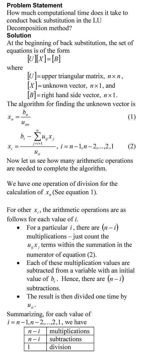
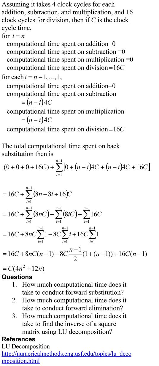
How much computational time does it take to find the inverse of a square matrix using Gauss Jordan method?  Part 1 of 2.

Problem Statement

How much computational time does it take to find the inverse of a square matrix using Gauss Jordan method?  Part 1 of 2.

Solution

To understand the solution, you should be familiar with the Gauss Jordan method of finding the inverse of a square matrix.  Peter Young of UCSC describes it briefly in this pdf file while if you like watching an example via a video, you can see PatrickJMT doing so.  You also need to read a previous blog where we calculated the computational time needed for the forward elimination steps on a square matrix in the Naïve Gauss elimination method.   We are now ready to estimate the computational time required for Gauss Jordan method of finding the inverse of a square matrix.

GJ Inverse Blog

This post is brought to you by

Computational Time for Forward Elimination Steps of Naive Gaussian Elimination on a Square Matrix

Problem Statement

How much computational time does it take to conduct the forward elimination part of the Naïve Gauss Elimination method on a square matrix?

CTdecomposition

This post is brought to you by

Computational Time to Find Determinant Using Gaussian Elimination

The time it would take to find the determinant of a matrix using the Gaussian Elimination is many-many orders less than when the cofactor method is used.  In this blog, we derive the formula for a typical amount of computational time it would take to find the determinant of a nxn matrix using the forward elimination part of the Naive Gauss Elimination method.  The time is compared with that using the cofactor method.
 Computational time to find determinant

Computational time to find determinant

This post is brought to you by Holistic Numerical Methods: Numerical Methods for the STEM undergraduate at http://nm.mathforcollege.com, the textbook on Numerical Methods with Applications available from the lulu storefront, the textbook on Introduction to Programming Concepts Using MATLAB, and the YouTube video lectures available at http://nm.mathforcollege.com/videos.  Subscribe to the blog via a reader or email to stay updated with this blog. Let the information follow you.

Computational Time to Find Determinant Using CoFactor Method

The time it would take to find the determinant of a matrix using the cofactor method can be daunting.  A student may not realize this as they may be limited to finding determinants of matrices of order 4×4 or less by hand.  In this blog, we derive the formula for a typical amount of computational time it would take to find the determinant of a nxn matrix using the cofactor method.
 Computational time to find determinant

Computational time to find determinant

This post is brought to you by Holistic Numerical Methods: Numerical Methods for the STEM undergraduate at http://nm.mathforcollege.com, the textbook on Numerical Methods with Applications available from the lulu storefront, the textbook on Introduction to Programming Concepts Using MATLAB, and the YouTube video lectures available at http://nm.mathforcollege.com/videos.  Subscribe to the blog via a reader or email to stay updated with this blog. Let the information follow you.

Computational Time for Forward Substitution

In the previous blog, we found the computatational time for back substitution. This is a blog that will show you how we can find the approximate time it takes to conduct forward substitution, while solving simultaneous linear equations. The blog assumes a AMD-K7 2.0GHz chip that uses 4 clock cycles for addition, subtraction and multiplication, while 16 clock cycles for division. Note that we are making reasonable approximations in this blog. Our main motto is to see what the computational time is proportional to – does the computational time double or quadruple if the number of equations is doubled.

Forward Substitution Time

The pdf file of the solution is also available.

This post is brought to you by

Subscribe to the blog via a reader or email to stay updated with this blog. Let the information follow you.

Computational Time for Back Substitution

This is a blog that will show you how we can find the approximate time it takes to conduct back substitution, while solving simultaneous linear equations using Gaussian elimination method. The blog assumes a AMD-K7 2.0GHz chip that uses 4 clock cycles for addition, subtraction and multiplication, and 16 clock cycles for division. Note that we are making reasonable approximations in this blog. Our main motto is to find how the computational time is related to the number of equations.

The pdf file of the solution is also available.

This post is brought to you by

Subscribe to the blog via a reader or email to stay updated with this blog. Let the information follow you.

So what does this mean that the computational time is proportional to some power of n in Gaussian Elimination method?

In a previous post, we talked about why LU Decomposition is computationally more efficient than Gaussian Elimination in some cases. The argument was based on how much computational time does each of the methods take. For example, we said that for back substitution in both methods, the computational time is approximately proportional to $latex n^2/2$.

How did we find that for back substitution the computational time is approximately proportional to $latex n^2/2$?

The amount of time it takes to conduct back substitution depends on the number of floating point operations (FLOPs) needed. Depending on how many FLOPs the computer can execute in a second called FLOPS (note the upper case S to distinguish between FLOPs and FLOPS), that will the determine the actual computational time. (A typical Pentium 4 PC conducts to the order of $latex 10^{9}$ FLOPS; a state-of-art supercomputer conducts to the order of $latex 10^{15}$ FLOPS; in 1983 the PC with a 8087 chip may have conducted to the order of $latex 10^{5}$ FLOPS).

To keep things simple, let’s only count the multiplication/division FLOPs in back substitution as time used by multiplication and division is higher than addition and subtraction (Multiplication may take twice and division as much as thrice the time it takes for addition and subtraction).

In back substitution, we start with the last equation. The last equation involves one division, second last equation involves one multiplication and one division, the third last equation involves two multiplications and one division, and so on. So the number of multiplication/divisions FLOPs is 1 for last equation, 2 for second last equation, 3 for third last equation, that is, for all equations, $latex 1+2….+n=n^2/2+n/2 $. For large n, this number is approximately $latex n^2/2$.

This post brought to you by Holistic Numerical Methods: Numerical Methods for the STEM undergraduate at http://nm.mathforcollege.com