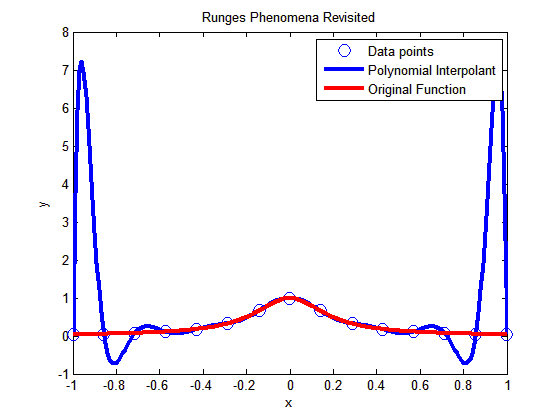
In a previous post, we talked about that higher order interpolation is a bad idea.

In this post I am showing you a MATLAB program that will allow you to experiment by changing the number of data points you choose, that is, the value of n (see the input highlighted in red in the code – this is the only line you want to change) and see for yourself why high order interpolation is a bad idea. Just, cut and paste the code below (or download it from http://www.eng.usf.edu/~kaw/download/runge.m) in the MATLAB editor and run it.
% Simulation : Higher Order Interpolation is a Bad Idea
% Language : Matlab r12
% Authors : Autar Kaw
% Last Revised : June 10 2008
% Abstract: In 1901, Carl Runge published his work on dangers of high order
% interpolation. He took a simple looking function f(x)=1/(1+25x^2) on
% the interval [-1,1]. He took points equidistantly spaced in [-1,1]
% and interpolated the points with polynomials. He found that as he
% took more points, the polynomials and the original curve differed
% even more considerably. Try n=5 and n=25
clc
clear all
clf
disp(‘In 1901, Carl Runge published his work on dangers of high order’)
disp(‘interpolation. He took a simple looking function f(x)=1/(1+25x^2) on’)
disp(‘the interval [-1,1]. He took points equidistantly spaced in [-1,1]’)
disp(‘and interpolated the points with a polynomial. He found that as he’)
disp(‘took more points, the polynomials and the original curve differed’)
disp(‘even more considerably. Try n=5 and n=15’)
%
% INPUT:
% Enter the following
% n= number of equidisant x points from -1 to +1
n=15;
% SOLUTION
disp(‘ ‘)
disp(‘SOLUTION’)
disp(‘Check out the plots to appreciate: High order interpolation is a bad idea’)
fprintf(‘\nNumber of data points used =%g’,n)
% h = equidisant spacing between points
h=2.0/(n-1);
syms xx
% generating n data points equally spaced along the x-axis
% First data point
x(1)=-1;
y(1)=subs(1/(1+25*xx^2),xx,-1);
% Other data points
for i=2:1:n
x(i)=x(i-1)+h;
y(i)=subs(1/(1+25*xx^2),xx,x(i));
end
% Generating the (n-1)th order polynomial from the n data points
p=polyfit(x,y,n-1);
% Generating the points on the polynomial for plotting
xpoly=-1:0.01:1;
ypoly=polyval(p,xpoly);
% Generating the points on the function itself for plotting
xfun=-1:0.01:1;
yfun=subs(1/(1+25*xx^2),xx,xfun);
% The classic plot
% Plotting the points
plot(x,y,’o’,’MarkerSize’,10)
hold on
% Plotting the polynomial curve
plot(xpoly,ypoly,’LineWidth’,3,’Color’,’Blue’)
hold on
% Plotting the origianl function
plot(xfun,yfun,’LineWidth’,3,’Color’,’Red’)
hold off
xlabel(‘x’)
ylabel(‘y’)
title(‘Runges Phenomena Revisited’)
legend(‘Data points’,’Polynomial Interpolant’,’Original Function’)
%***********************************************************************
disp(‘ ‘)
disp(‘ ‘)
disp(‘What you will find is that the polynomials diverge for’)
disp(‘0.726<|x|<1. If you started to choose same number of points ‘)
disp(‘but more of them close to -1 and +1, you would avoid such divergence. ‘)
disp(‘ ‘)
disp(‘However, there is no general rule to pick points for a general ‘)
disp(‘function so that this divergence is avoided; but some rules do exist for ‘)
disp(‘certian types of functions.’)
This post is brought to you by Holistic Numerical Methods: Numerical Methods for the STEM undergraduate at http://nm.mathforcollege.com