Does the solve command in MATLAB not give you an answer?

In a recent blog about the MATLAB solve command, I mentioned that the solve command was not giving us the unique real solution to a physical problem.  A user at MATLAB suggested declaring the syms variable as real, before using the solve command. That worked.  So if the equation in terms of the variable b is eqnb=0, then use

syms b real;
solve (eqnb,b);

____________________________________________
This post is brought to you by Holistic Numerical Methods: Numerical Methods for the STEM undergraduate at http://nm.mathforcollege.com, the textbook on Numerical Methods with Applications available from the lulu storefront, the textbook on Introduction to Programming Concepts Using MATLAB, and the YouTube video lectures available athttp://nm.mathforcollege.com/videos.  Subscribe to the blog via a reader or email to stay updated with this blog. Let the information follow you.

Computational Time to Find Determinant Using Gaussian Elimination

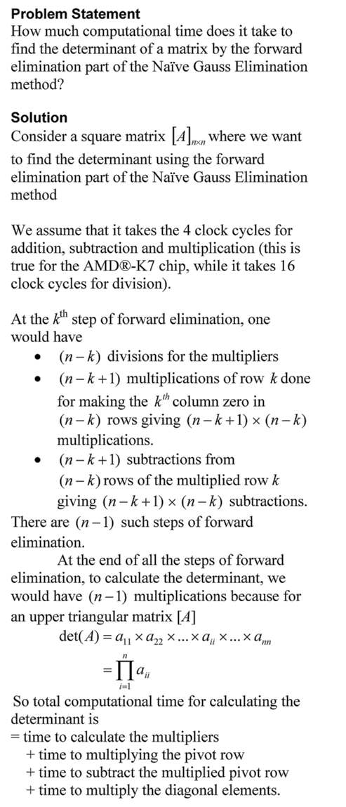
The time it would take to find the determinant of a matrix using the Gaussian Elimination is many-many orders less than when the cofactor method is used.  In this blog, we derive the formula for a typical amount of computational time it would take to find the determinant of a nxn matrix using the forward elimination part of the Naive Gauss Elimination method.  The time is compared with that using the cofactor method.
 Computational time to find determinant

Computational time to find determinant

This post is brought to you by Holistic Numerical Methods: Numerical Methods for the STEM undergraduate at http://nm.mathforcollege.com, the textbook on Numerical Methods with Applications available from the lulu storefront, the textbook on Introduction to Programming Concepts Using MATLAB, and the YouTube video lectures available at http://nm.mathforcollege.com/videos.  Subscribe to the blog via a reader or email to stay updated with this blog. Let the information follow you.

Does the solve command in MATLAB not give you an answer?

Recently, I had assigned a project to my class where they needed to regress n number of x-y data points to a nonlinear regression model y=exp(b*x).  However, they were NOT allowed to transform the data, that is, transform data such that linear regression formulas can be used to find the constant of regression b.  They had to do it the new-fashioned way: Find the sum of the square of the residuals and then minimize the sum with respect to the constant of regression b.

To do this, they conducted the following steps

  1. setup the equation by declaring b as a syms variable,
  2. calculate the sum  of the square of the residuals using a loop,
  3. use the diff command to set up the equation,
  4. use the solve command. 

However, the solve command gave some odd answer like log(z1)/5 + (2*pi*k*i)/5.  The students knew that the equation has only one real solution – this was deduced from the physics of the problem. 

We did not want to set up a separate function mfile to use the numerical solvers such as fsolve.  To circumvent the setting up of a separate function mfile, we approached it as follows.  If dbsr=0 is the equation you want to solve, use

F = vectorize(inline(char(dbsr)))
fsolve(F, -2.0)

What char command does is to convert the function dbsr to a string, inline constructs it to an inline function, vectorize command vectorizes the formula (I do not fully understand this last part myself or whether it is needed).

This post is brought to you by Holistic Numerical Methods: Numerical Methods for the STEM undergraduate at http://nm.mathforcollege.com, the textbook on Numerical Methods with Applications available from the lulu storefront, the textbook on Introduction to Programming Concepts Using MATLAB, and the YouTube video lectures available athttp://nm.mathforcollege.com/videos.  Subscribe to the blog via a reader or email to stay updated with this blog. Let the information follow you.

Computational Time to Find Determinant Using CoFactor Method

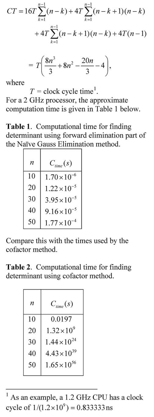
The time it would take to find the determinant of a matrix using the cofactor method can be daunting.  A student may not realize this as they may be limited to finding determinants of matrices of order 4×4 or less by hand.  In this blog, we derive the formula for a typical amount of computational time it would take to find the determinant of a nxn matrix using the cofactor method.
 Computational time to find determinant

Computational time to find determinant

This post is brought to you by Holistic Numerical Methods: Numerical Methods for the STEM undergraduate at http://nm.mathforcollege.com, the textbook on Numerical Methods with Applications available from the lulu storefront, the textbook on Introduction to Programming Concepts Using MATLAB, and the YouTube video lectures available at http://nm.mathforcollege.com/videos.  Subscribe to the blog via a reader or email to stay updated with this blog. Let the information follow you.

A MATLAB program to find quadrature points and weights for Gauss-Legendre Quadrature rule

Recently, I got a request how one can find the quadrature and weights of a Gauss-Legendre quadrature rule for large n.  It seems that the internet has these points available free of charge only up to n=12.  Below is the MATLAB program that finds these values for any n.  I tried the program for n=25 and it gave results in a minute or so.  The results output up to 32 significant digits.
_______________________________________________________
% Program to get the quadrature points
% and weight for Gauss-Legendre Quadrature
% Rule
clc
clear all
syms x
% Input n: Quad pt rule
n=14;
% Calculating the Pn(x)
% Legendre Polynomial
% Using recursive relationship
% P(order of polynomial, value of x)
% P(0,x)=1; P(1,x)=0;
% (i+1)*P(i+1,x)=(2*i+1)*x*P(i,x)-i*P(i-1,x)
m=n-1;
P0=1;
P1=x;
for i=1:1:m
    Pn=((2.0*i+1)*x*P1-i*P0)/(i+1.0);
    P0=P1;
    P1=Pn;
end
if n==1
    Pn=P1;
end
Pn=expand(Pn);
quadpts=solve(vpa(Pn,32));
quadpts=sort(quadpts);
% Finding the weights
% Formula for weights is given at
% http://mathworld.wolfram.com/Legendre-GaussQuadrature.html
% Equation (13)
for k=1:1:n
    P0=1;
    P1=x;
    m=n;
    % Calculating P(n+1,x)
    for i=1:1:m
        Pn=((2.0*i+1)*x*P1-i*P0)/(i+1.0);
        P0=P1;
        P1=Pn;
    end
    Pn=P1;
    weights(k)=vpa(2*(1-quadpts(k)^2)/(n+1)^2/ …
                                   subs(Pn,x,quadpts(k))^2,32);
end
    fprintf(‘Quad point rule for n=%g \n’,n)
disp(‘  ‘)
disp(‘Abscissas’)
disp(quadpts)
disp(‘  ‘)
disp(‘Weights’)
disp(weights’)_______________________________________________________ 

This post is brought to you by Holistic Numerical Methods: Numerical Methods for the STEM undergraduate at http://nm.mathforcollege.com, the textbook on Numerical Methods with Applications available from the lulu storefront, the textbook on Introduction to Programming Concepts Using MATLAB, and the YouTube video lectures available at http://nm.mathforcollege.com/videos.  Subscribe to the blog via a reader or email to stay updated with this blog. Let the information follow you.

YouTube Videos on Numerical Methods Cross 1-Million Views Mark

In a short 2.5 years since starting the numericalmethodsguy YouTube channel in January 2009, this month the channel crossed the benchmark of receiving 1 million video views.  Currently the channel gets between 2,500-3,500 video views per day.  Although we have playlists on the channel, the playlist for all the available topics are given on single webpage at http://nm.mathforcollege.com/videos/index.html

Complete resources on each topic of available numerical methods including textbook chapters, videos, multiple-choice tests, PPTs, and worksheets are  given at http://nm.mathforcollege.com/topics/textbook_index.html
__________________________________________________

This post is brought to you by Holistic Numerical Methods: Numerical Methods for the STEM undergraduate at http://nm.mathforcollege.com, the textbook on Numerical Methods with Applications available from the lulu storefront, the textbook on Introduction to Programming Concepts Using MATLAB, and the YouTube video lectures available at http://nm.mathforcollege.com/videos.  Subscribe to the blog via a reader or email to stay updated with this blog. Let the information follow you.

A Wolfram demo on how much of a floating ball is under water

Here is another Wolfram demo. This one shows how much of a floating ball would be submerged under water.  The demonstration uses the specific gravity and radius of the ball as inputs.  Using calculus and Archimedes’ principle, the level to which the ball is submerged turns out to be the solution of a cubic equation.  To play with the demo, download the free CDF player from Wolfram first.


This post is brought to you by Holistic Numerical Methods: Numerical Methods for the STEM undergraduate at http://nm.mathforcollege.com, the textbook on Numerical Methods with Applications available from the lulu storefront, the textbook on Introduction to Programming Concepts Using MATLAB, and the YouTube video lectures available at http://nm.mathforcollege.com/videos.  Subscribe to the blog via a reader or email to stay updated with this blog. Let the information follow you.

Order of accuracy of central divided difference scheme for first derivative of a function of one variable

This post is brought to you by
Holistic Numerical Methods: Numerical Methods for the STEM undergraduate at http://nm.mathforcollege.com, the textbook on Numerical Methods with Applications available from the lulu storefront, the textbook on Introduction to Programming Concepts Using MATLAB, and the YouTube video lectures available at http://nm.mathforcollege.com/videos.  Subscribe to the blog via a reader or email to stay updated with this blog. Let the information follow you.

A Wolfram demo on converting a decimal number to floating point binary representation

Here is another Wolfram demo. This one converts a decimal number to a floating point binary representation.  To play with the demo, download the free CDF player first.
 
The total number of bits used for the representation =
       one bit for the sign of the number +
       one bit for the sign of the exponent +
       number of bits for the exponent +
       number of bits for the mantissa +
       As an example, how would 54.75 be represented in a 9-bit register where the first bit is used for the sign of the number, second bit is used for sign of exponent, next three bits are used for the exponent, and the last four bits are used for the mantissa?
Both the number and the exponent are positive. 
As the number is normalized to lie between 1 and 2 (the interval being half-closed at the bottom and half-open at the top), the leading binary digit is always 1. So we do not actually use it in the representation of the mantissa. Hence the mantissa bits are 1011. Moreover the exponent bits are 101, the sign of the number bit is 0, and the sign of the exponent bit is 0.
Therefore the representation is .
 

Reference: Floating Point Representation

This post is brought to you by

Holistic Numerical Methods: Numerical Methods for the STEM undergraduate at http://nm.mathforcollege.com, the textbook on Numerical Methods with Applications available from the lulu storefront, the textbook on Introduction to Programming Concepts Using MATLAB, and the YouTube video lectures available at http://nm.mathforcollege.com/videos.  Subscribe to the blog via a reader or email to stay updated with this blog. Let the information follow you.