Making sense of the Big Oh!

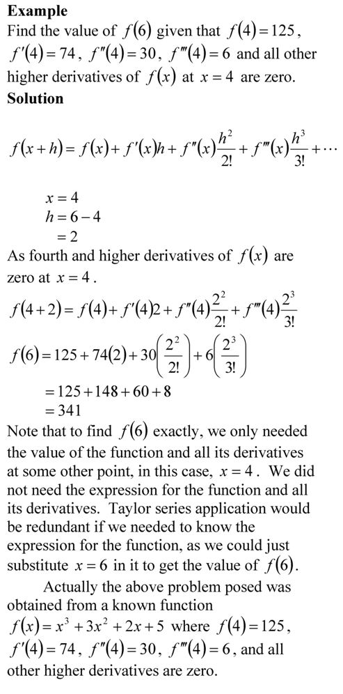
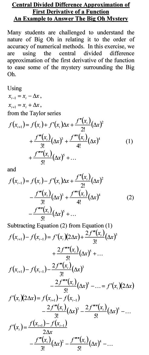
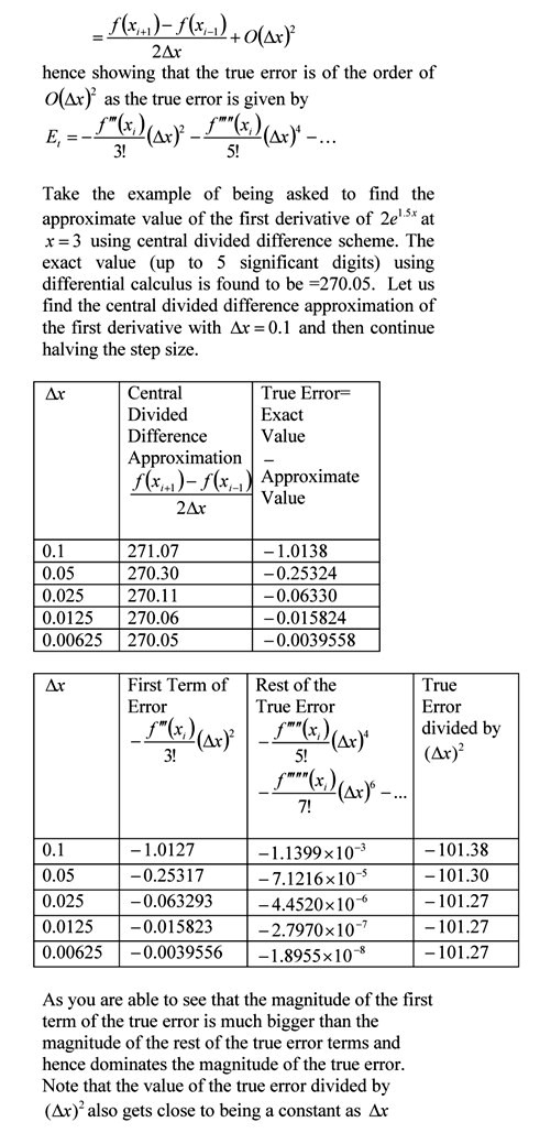
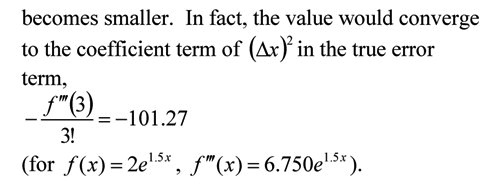
Many students are challenged to understand the nature of Big Oh in relating it to the order of accuracy of numerical methods.  In this exercise, we are using the central divided difference approximation of the first derivative of the function to ease some of the mystery surrounding the Big Oh.


You can visit the above example by opening a pdf file.

This post is brought to you by Holistic Numerical Methods: Numerical Methods for the STEM undergraduate at http://nm.MathForCollege.com, the textbook on Numerical Methods with Applications available from the lulu storefront, the textbook on Introduction to Programming Concepts Using MATLAB, and the YouTube video lectures available at http://nm.MathForCollege.com/videos.  Subscribe to the blog via a reader or email to stay updated with this blog. Let the information follow you.

Taylor series example

If Archimedes were to quote Taylor’s theorem, he would have said, “Give me the value of the function  and the value of all (first, second, and so on) its derivatives at a single point, and I can give you the value of the function at any other point”.

It is very important to note that the Taylor’s theorem is not asking for the expression of the function and its derivatives, just the value of the function and its derivatives at a single point.

Now the fine print: Yes, all the derivatives have to exist and be continuous between x and x+h, the point where you are wanting to calculate the function at. However, if you want to calculate the function approximately by using the nth order Taylor polynomial, then 1st, 2nd,…., nth derivatives need to exist and be continuous in the closed interval [x,x+h], while the (n+1)th derivative needs to exist and be continuous in the open interval (x,x+h).