Interpolation – Page 2 – Numerical Methods Guy

Do quadratic splines really use all the data points?

There are two reasons that linear splines are seldom used

Each spline uses information only from two consecutive data points
The slope of the splines is discontinuous at the interior data points

The answer to resolving the above concerns are to use higher order splines such as quadratic splines. Read the quadratic spline textbook notes before you go any further. You do want what I have to say to make sense to you.

In quadratic splines, a quadratic polynomial is assumed to go thru consecutive data points. So you cannot just find the three constants of each quadratic polynomial spline by using the information that the spline goes thru two consecutive points (that sets up two equations and three unknowns). Hence, we incorporate that the splines have a continuous slope at the interior points.

So does all this incorporation make the splines to depend on the values of all given data points. It does not seem so.

For example, in quadratic splines you have to assume that the first or last spline is linear. For argument sake, let that be the first spline. If the first spline is linear, then we can find the constants of the linear spline just by the knowledge of the value of the first two data points. So now we know that we can set up three equations for the three unknown constants of the second spline as follows

the slope of the first spline at the 2nd data point and the slope of the second spline at the 2nd point are the same,
the second spline goes thru the 2nd data point
the second spline goes thru the 3rd data point

That itself is enough information to find the three constants of the second spline. We can keep using the same argument for all the other splines.

So the mth spline constants are dependent on data from the data points 1, 2, .., m, m+1 but not beyond that.

Can you now make the call on the kind of dependence or independence you have in the constants of the quadratic splines?

This post is brought to you by Holistic Numerical Methods: Numerical Methods for the STEM undergraduate at http://nm.mathforcollege.com

Subscribe to the feed to stay updated and let the information follow you.

Extrapolation is inexact and may be dangerous

The NASDAQ was booming – people were dreaming of riches – early retirement and what not. The year was 1999 and NASDAQ was at an all time high of 4069 on the last day of 1999.

Yes, Prince was right, not just about the purple rain, but – “‘Cuz they say two thousand zero zero party over, Oops out of time, So tonight I’m gonna party like it’s 1999 party like 1999.”

But as we know the party did not last too long. The dot com bubble burst and as we know it today (June 2008), the NASDAQ is hovering around 2400.

Year ………………NASDAQ on December 31st

1994………………………… 751

1995 ……………………….1052

1996 ………………………..1291

1997 ………………………..1570

1998 ………………………..2192

1999 ………………………..4069

• End of Year NASDAQ Composite Data taken from www.bigcharts.com

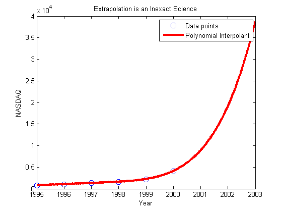
So how about extrapolating the value of NASDAQ to not too far ahead – just to the end of 2000 and 2001. This is what you obtain from using a 5th order interpolant for approximation from the above six values.

End of Year …Actual Value …..5th Order Poly Extrapo……………Abs Rel True Error
2000 ……………..2471…………………. 9128 ………………………………….. 269%
2001………………1950……………….. 20720 ………………………………….. 962%

Do you know what would be the extrapolated value of NASDAQ on June 30, 2008 -a whopping 861391! On June 30, 2008, compare it with the actual value.

This post is brought to you by Holistic Numerical Methods: Numerical Methods for the STEM undergraduate at http://nm.mathforcollege.com

Finding the length of curve using MATLAB

As per integral calculus, the length of a continuous and differentiable curve f(x) from x=a to x=b is given by

S= $\int_a^b \sqrt{(1+(dy/dx)^2} dx$

Now how do we find the length of a curve in MATLAB.

Let us do this via an example. Assume one asked you to find the length of $latex x^2*sin(x) $ from Π to 2Π. In the book, How People Learn, the authors mention that learning a concept in multiple contexts prolongs retention. Although it may not be the context that the authors of the book are talking about, let us find the length of the curve multiple ways within MATLAB. Try the program for functions and limits of your own choice to evaluate the difference.

METHOD 1: Use the formula S= $\int_a^b \sqrt{(1+(dy/dx)^2} dx$ by using the diff and int function of MATLAB

METHOD 2: Generate several points between a and b, and join straight lines between consecutive data points. Add the length of these straight lines to find the length of the curve.

METHOD 3. Find the derivative dy/dx numerically using forward divided difference scheme, and then use trapezoidal rule (trapz command in MATLAB) for discrete data with unequal segments to find the length of the curve.

QUESTIONS TO BE ANSWERED:

Why does METHOD 3 giving inaccurate results? Can you make them better by using better approximations of derivative like central divided difference scheme?
Redo the problem with f(x)= $x^{\frac{3}{2}}$ with a=1 and b=4 as the exact length can be found for such a function.

% Simulation : Find length of a given Curve
% Language : Matlab 2007a
% Authors : Autar Kaw
% Last Revised : June 14 2008
% Abstract: We are finding the length of the curve by three different ways
% 1. Using the formula from calculus
% 2. Breaking the curve into bunch of small straight lines
% 3. Finding dy/dx of the formula numerically to use discrete function
% integration
clc
clear all

disp(‘We are finding the length of the curve by three different ways’)
disp(‘1. Using the formula from calculus’)
disp(‘2. Breaking the curve into bunch of small straight lines’)
disp(‘3. Finding dy/dx of the formula numerically to use discrete function integration’)

%INPUTS – this is where you will change input data if you are doing
% a different problem
syms x;
% Define the function
curve=x^2*sin(x)
% lower limit
a=pi
% b=upper limit
b=2*pi
% n = number of straight lines used to approximate f(x) for METHOD 2
n=100
%p = number of discrete data points where dy/dx is calculated for METHOD 3
p=100

% OUTPUTS
% METHOD 1. Using the calculus formula
% S=int(sqrt(1+dy/dx^2),a,b)
% finding dy/dx
poly_dif=diff(curve,x,1);
% applying the formula
integrand=sqrt(1+poly_dif^2);
leng_exact=double(int(integrand,x,a,b));
fprintf (‘\nExact length =%g’,leng_exact)
%***********************************************************************

% METHOD 2. Breaking the curve as if it is made of small length
% straight lines
% Generating n x-points from a to b

xi= a:(b-a)/n:b;
% generating the y-values of the function
yi=subs(curve,x,xi);
% assuming that between consecutive data points, the
% curve can be approximated by linear splines.
leng_straight=0;
m=length(xi);
% there are m-1 splines for m points
for i=1:1:m-1
dx=xi(i+1)-xi(i);
dy= yi(i+1)-yi(i);
leneach=sqrt(dx^2+dy^2);
leng_straight=leng_straight+leneach;
end
fprintf (‘\n\nBreaking the line into short lengths =%g’,leng_straight)

% METHOD 3. Same as METHOD1, but calculating dy/dx
% numerically and integrating using trapz
xi=a:(b-a)/p:b;
% generating the dy/dx-values
m=length(xi);
for i=1:1:m-1
numer=yi(i+1)-yi(i);
den=xi(i+1)-xi(i);
dydxv(i)=numer/den;
end
% derivative at last point using Backward divided difference formula
% is same as Forward divided difference formula
dydxv(m)=dydxv(m-1);
integrandi=sqrt(1+dydxv.*dydxv);
length_fdd=trapz(xi,integrandi);
disp(‘ ‘)
disp(‘ ‘)
disp (‘Using numerical value of dy/dx coupled’)
disp (‘with discrete integration’)
fprintf (‘ =%g’,length_fdd)

This post is brought to you by Holistic Numerical Methods: Numerical Methods for the STEM undergraduate at http://nm.mathforcollege.com

A simple MATLAB program to show that High order interpolation is a bad idea

In a previous post, we talked about that higher order interpolation is a bad idea.

Runge's function

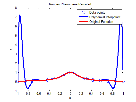
In this post I am showing you a MATLAB program that will allow you to experiment by changing the number of data points you choose, that is, the value of n (see the input highlighted in red in the code – this is the only line you want to change) and see for yourself why high order interpolation is a bad idea. Just, cut and paste the code below (or download it from http://www.eng.usf.edu/~kaw/download/runge.m) in the MATLAB editor and run it.

% Simulation : Higher Order Interpolation is a Bad Idea

% Language : Matlab r12
% Authors : Autar Kaw
% Last Revised : June 10 2008
% Abstract: In 1901, Carl Runge published his work on dangers of high order
% interpolation. He took a simple looking function f(x)=1/(1+25x^2) on
% the interval [-1,1]. He took points equidistantly spaced in [-1,1]
% and interpolated the points with polynomials. He found that as he
% took more points, the polynomials and the original curve differed
% even more considerably. Try n=5 and n=25
clc
clear all
clf

disp(‘In 1901, Carl Runge published his work on dangers of high order’)
disp(‘interpolation. He took a simple looking function f(x)=1/(1+25x^2) on’)
disp(‘the interval [-1,1]. He took points equidistantly spaced in [-1,1]’)
disp(‘and interpolated the points with a polynomial. He found that as he’)
disp(‘took more points, the polynomials and the original curve differed’)
disp(‘even more considerably. Try n=5 and n=15’)

%
% INPUT:
% Enter the following
% n= number of equidisant x points from -1 to +1
n=15;

% SOLUTION
disp(‘ ‘)
disp(‘SOLUTION’)
disp(‘Check out the plots to appreciate: High order interpolation is a bad idea’)
fprintf(‘\nNumber of data points used =%g’,n)
% h = equidisant spacing between points
h=2.0/(n-1);
syms xx
% generating n data points equally spaced along the x-axis
% First data point
x(1)=-1;
y(1)=subs(1/(1+25*xx^2),xx,-1);
% Other data points
for i=2:1:n
x(i)=x(i-1)+h;
y(i)=subs(1/(1+25*xx^2),xx,x(i));
end

% Generating the (n-1)th order polynomial from the n data points
p=polyfit(x,y,n-1);

% Generating the points on the polynomial for plotting
xpoly=-1:0.01:1;
ypoly=polyval(p,xpoly);

% Generating the points on the function itself for plotting
xfun=-1:0.01:1;
yfun=subs(1/(1+25*xx^2),xx,xfun);

% The classic plot
% Plotting the points
plot(x,y,’o’,’MarkerSize’,10)
hold on
% Plotting the polynomial curve
plot(xpoly,ypoly,’LineWidth’,3,’Color’,’Blue’)
hold on
% Plotting the origianl function
plot(xfun,yfun,’LineWidth’,3,’Color’,’Red’)
hold off
xlabel(‘x’)
ylabel(‘y’)
title(‘Runges Phenomena Revisited’)
legend(‘Data points’,’Polynomial Interpolant’,’Original Function’)
%***********************************************************************
disp(‘ ‘)
disp(‘ ‘)
disp(‘What you will find is that the polynomials diverge for’)
disp(‘0.726<|x|<1. If you started to choose same number of points ‘)
disp(‘but more of them close to -1 and +1, you would avoid such divergence. ‘)
disp(‘ ‘)
disp(‘However, there is no general rule to pick points for a general ‘)
disp(‘function so that this divergence is avoided; but some rules do exist for ‘)
disp(‘certian types of functions.’)

This post is brought to you by Holistic Numerical Methods: Numerical Methods for the STEM undergraduate at http://nm.mathforcollege.com

High order interpolation is a bad idea?

One would intuitively assume that if one was given 100 data points of data, it would be most accurate to interpolate the 100 data points to a 99th order polynomial. More the merrier: is that not the motto. But I am sorry to burst your bubble – high order interpolation is generally a bad idea.

The classic example (dating as back as 1901 before there were calculators) to show that higher order interpolation idea is a bad idea comes from the famous German mathematician Carl Runge.

He took a simple and smooth function, f(x) = 1/(1+25x^2) in the domain [-1,1]. He chose equidisant x-data points on the function f(x) in the domain xε[-1,1]. Then he used those data points to draw a polynomial interpolant.

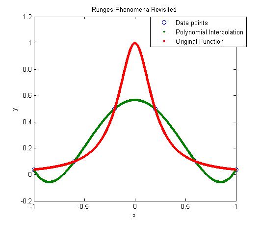
For example, if I chose 6 data points equidistantly spaced on [-1,1], those are (-1, 0.038462), (-0.6, 0.1), (-0.2,0.5), (0.2,0.5), (0.6,0.1), and (1,0.038462). I can interpolate these 6 data points by a 5th order polynomial. In Figure 1, I am then plotting the fifth order polynomial and the original function. You can observe that there is a large difference between the original function and the polynomial interpolant. The polynomial does go through the six points, but at many other points it does not even come close to the original function. Just look at x= 0.85, the value of the function is 0.052459, but the fifth order polynomial gives you a value of -0.055762, a whopping 206.30 % error; also note the opposite sign.

Figure 1. 5th order polynomial interpolation with six equidistant points.

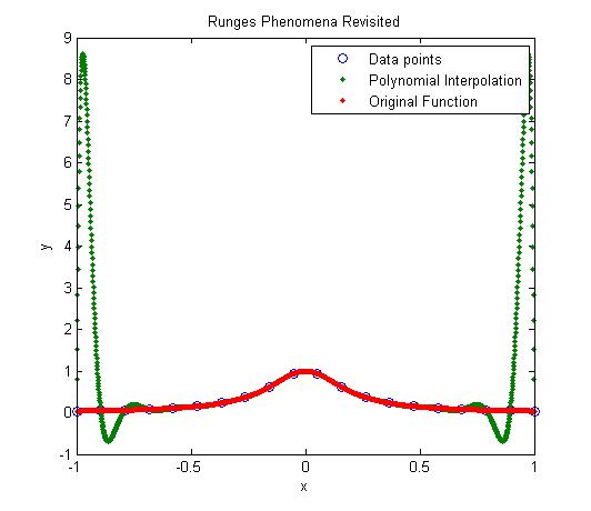
Maybe I am not taking enough data points. Six points may be too small a number to approximate the function. Ok! Let’s get crazy. How about 20 points? That will give us a 19th order polynomial. I will choose 20 points equidistantly in [-1,1].

Figure 2. 19th order polynomial interpolation with twenty equidistant points

It is not any better though it did do a better job of approximating the function except near the ends. At the ends, it is worse than before. At our chosen point, x= 0.85, the value of the function is 0.052459, while we get -0.62944 from the 19th order polynomial, and that is a big whopper error of 1299.9 %.

So are you convinced that higher order interpolation is a bad idea? Try an example by yourself: step function y=-1, -1<x<0 and y=+1, 0<x<1.

What is the alternative to higher order interpolation? Is it lower order interpolation, but does that not use data only from less points than are given. How can we use lower order polynomials and at the same time use information from all the given data points. The answer to that question is SPLINE interpolation.

This post is brought to you by Holistic Numerical Methods: Numerical Methods for the STEM undergraduate at http://nm.mathforcollege.com

If a polynomial of order n or less passes thru (n+1) points, it is unique!

Given n+1 (x,y) data pairs, with all x values being unique, then a polynomial of order n or less passes thru the (n+1) data points. How can we prove that this polynomial is unique?

I am going to show you the proof for a particular case and you can extend it to polynomials of any order n.

Lets suppose you are given three data points (x1,y1), (x2,y2), (x3,y3) where x1 $\ne$ x2 $\ne$ x3.

Then if a polynomial P(x) of order 2 or less passes thru the three data points, we want to show that P(x) is unique.

We will prove this by contradiction.

Let there be another polynomial Q(x) of order 2 or less that goes thru the three data points. Then R(x)=P(x)-Q(x) is another polynomial of order 2 or less. But the value of P(x) and Q(x) is same at the three x-values of the data points x1, x2, x3. Hence R(x) has three zeros, at x=x1, x2 and x3.

But a second order polynomial only has two zeros; the only case where a second order polynomial can have three zeros is if R(x) is identically equal to zero, and hence have infinite zeros. Since R(x)=P(x)-Q(x), and R(x) $\equiv$ 0, then P(x) $\equiv$ Q(x). End of proof.

But how do you know that a second order polynomial with three zeros is identically zero.

R(x) is of the form a0+a1*x+a2*x^2 and has three zeros, x1, x2, x3. Then it needs to satisfy the following three equations

a0+a1*x1+a2*x1^2=0

a0+a1*x2+a2*x2^2=0

a0+a1*x3+a2*x3^2=0

The above equations have the trivial solution a0=a1=a2=0 as the only solution if

det(1 x1 x1^2; 1 x2 x2^2; 1 x3 x3^2) $\ne$ 0.

That is in fact the case as

det(1 x1 x1^2; 1 x2 x2^2; 1 x3 x3^2) = (x1-x2)*(x2-x3)*(x3-x1),

and since x1 $\ne$ x2 $\ne$ x3, the

det(1 x1 x1^2; 1 x2 x2^2; 1 x3 x3^2) $\ne$ 0

So the only solution is a0=a1=a2=0 making R(x) $\equiv$ 0

This post brought to you by Holistic Numerical Methods: Numerical Methods for the STEM undergraduate at http://nm.mathforcollege.com