Ordinary Differential Equations – Page 2

Example: Solving First Order Linear ODE by Integrating Factor

I have a audiovisual digital lecture on YouTube that shows the use of Euler’s method to solve a first order ordinary differential equation (ODE). To show the accuracy of Euler’s method, I compare the approximate answer to the exact answer. A YouTube viewer asked me: How did I get the exact answer?

In this blog, I use the integrating factor method to find the exact answer, because that is the method the viewer was using to solve the ODE exactly. So here it is and in two future blogs, I will show the same example being solved by 1) Laplace transforms and 2) the classical (complementary + particular) solution techniques.
Solving First Order Linear ODE by Integrating Factor

The pdf file of the solution is also available.

This post is brought to you by

Holistic Numerical Methods: Numerical Methods for the STEM undergraduate at http://nm.mathforcollege.com,
the textbook on Numerical Methods with Applications available from the lulu storefront,
the textbook on Introduction to Programming Concepts Using MATLAB, and
the YouTube video lectures available at http://nm.mathforcollege.com/videos

Subscribe to the blog via a reader or email to stay updated with this blog. Let the information follow you.

How do I numerically solve an ODE in MATLAB?

The other day a student came to ask me for help in solving a second order ordinary differential equation using the ode45 routine of MATLAB. To use ode45, one needs to be familiar with how the inputs are required by MATLAB. The understanding of these inputs is important to use ode45 successfully in problems that are more complex than solving a second order ODE.

The ordinary differential equation was
2y”+3y’+5y=7 exp(-x), y(0)=11, dy/dx(0)=13
This has to put in the state variable form by reducing it by using
y’=z
That gives
y’=z with the corresponding initial conditions as y(0)=11
Then
2y”+3y’+5y=7 exp(-x)
reduces to
2z’ + 3z+5y=7exp(-x)
z’ =(7exp(-x)-3z-5y)/2 with the corresponding initial conditions as z(0)=13

So as needed by MATLAB, call y as y(1) and z as y(2)
dy(1)=y(2), y(1) at x=0 is 11
dy(2)=(7exp(-x)-3y(2)-5y(1))/2, y(2) at x=0 is 13

These equations are now put in a MATLAB function we call odestate.m
dy=zeros(2,1);
dy(1)=y(2);
dy(2)=(7*exp(-x)-3*y(2)-5*y(1))/2;

To solve the ODE, the
The inputs are
1) the function odestate
2) The outputs are required between x=0 and x=17,
hence entered as [0 17]
3) The initial conditions are y(0)=11 and dy/dx(0)=13,
hence entered as [11 13]

The outputs are
1) X= array of x values between 0 and 17
2) Y= matrix of 2 columns;
first column is the y(x)
second column is dy/dx(x)
The MATLAB code then is
[X,Y]=ode45(@odestate,[0 17],[11 13]);

Click the links for the MATLAB mfiles for the function odestate.m and the ODE solver odetest.m

_________________________________________________________________________________

This post is brought to you by Holistic Numerical Methods: Numerical Methods for the STEM undergraduate at http://nm.mathforcollege.com, the textbook on Numerical Methods with Applications available from the lulu storefront, and the YouTube video lectures available at http://nm.mathforcollege.com/videos and http://www.youtube.com/numericalmethodsguy

Subscribe to the blog via a reader or email to stay updated with this blog. Let the information follow you

How do I solve a boundary value ODE in MATLAB?

Many students ask me how do I do this or that in MATLAB. So I thought why not have a small series of my next few blogs do that. In this blog, I show you how to solve a boundary value ordinary differential equation.

The MATLAB program link is here.
The HTML version of the MATLAB program is here.
DO NOT COPY AND PASTE THE PROGRAM BELOW BECAUSE THE SINGLE QUOTES DO NOT TRANSLATE TO THE CORRECT SINGLE QUOTES IN MATLAB EDITOR. DOWNLOAD THE MATLAB PROGRAM INSTEAD

%% HOW DO I DO THAT IN MATLAB SERIES?
% In this series, I am answering questions that students have asked
% me about MATLAB. Most of the questions relate to a mathematical
% procedure.

%% TOPIC
% How do I solve a boundary value ordinary differential equation?

%% SUMMARY

% Language : Matlab 2008a;
% Authors : Autar Kaw;
% Mfile available at
% http://nm.mathforcollege.com/blog/ode_boundaryvalue.m;
% Last Revised : May 26, 2009;
% Abstract: This program shows you how to solve an
% boundary value ordinary differential equation.
clc
clear all

%% INTRODUCTION

disp(‘ABSTRACT’)
disp(‘   This program shows you how to solve’)
disp(‘   a boundary value ordinary differential equation’)
disp(‘ ‘)
disp(‘AUTHOR’)
disp(‘   Autar K Kaw of http://autarkaw.wordpress.com’)
disp(‘ ‘)
disp(‘MFILE SOURCE’)
disp(‘   http://nm.mathforcollege.com/blog/ode_boundaryvalue.m’)
disp(‘ ‘)
disp(‘LAST REVISED’)
disp(‘   May 26, 2009’)
disp(‘ ‘)

%% INPUTS
% Solve the ordinary differential equation
% y”-0.0000002y=0.000000075*x*(75-x)
% Define x as a symbol
syms x
%The ODE
ode_eqn=’D2y-0.000002*y=0.000000075*x*(75-x)’;
% The initial conditions
iv_1=’y(0)=0′;
iv_2=’y(75)=0′;
% The value at which y is sought at
xval=37.5;
%% DISPLAYING INPUTS

disp(‘INPUTS’)
func=[‘ The ODE to be solved is ‘ ode_eqn];
disp(func)
iv_explain=[‘ The boundary conditions are ‘ iv_1 ‘ ‘ iv_2];
disp(iv_explain)
fprintf(‘ The value of y is sought at x=%g’,xval)
disp(‘ ‘)

%% THE CODE

% Finding the solution of the ordinary differential equation
soln=dsolve(ode_eqn,iv_1,iv_2,’x’);
% vpa below uses variable-precision arithmetic (VPA) to compute each
% element of soln to 5 decimal digits of accuracy
soln=vpa(soln,5);

%% DISPLAYING OUTPUTS
disp(‘ ‘)
disp(‘OUTPUTS’)
output=[‘ The solution to the ODE is ‘ char(soln)];
disp(output)
value=subs(soln,x,xval);
fprintf(‘ The value of y at x=%g is %g’,xval,value)
disp(‘ ‘)

Subscribe to the blog via a reader or email to stay updated with this blog. Let the information follow you.

How do I solve an initial value ODE in MATLAB?

Many students ask me how do I do this or that in MATLAB. So I thought why not have a small series of my next few blogs do that. In this blog, I show you how to solve an initial value ordinary differential equation.

The MATLAB program link is here.
The HTML version of the MATLAB program is here.
DO NOT COPY AND PASTE THE PROGRAM BELOW BECAUSE THE SINGLE QUOTES DO NOT TRANSLATE TO THE CORRECT SINGLE QUOTES IN MATLAB EDITOR. DOWNLOAD THE MATLAB PROGRAM INSTEAD

%% HOW DO I DO THAT IN MATLAB SERIES?
% In this series, I am answering questions that students have asked
% me about MATLAB. Most of the questions relate to a mathematical
% procedure.

%% TOPIC
% How do I solve an initial value ordinary differential equation?

%% SUMMARY

% Language : Matlab 2008a;
% Authors : Autar Kaw;
% Mfile available at
% http://nm.mathforcollege.com/blog/ode_initial.m;
% Last Revised : May 14, 2009;
% Abstract: This program shows you how to solve an
% initial value ordinary differential equation.
clc
clear all

%% INTRODUCTION

disp(‘ABSTRACT’)
disp(‘   This program shows you how to solve’)
disp(‘   an initial value ordinary differential equation’)
disp(‘ ‘)
disp(‘AUTHOR’)
disp(‘   Autar K Kaw of http://autarkaw.wordpress.com’)
disp(‘ ‘)
disp(‘MFILE SOURCE’)
disp(‘   http://nm.mathforcollege.com/blog/ode_initial.m’)
disp(‘ ‘)
disp(‘LAST REVISED’)
disp(‘   May 14, 2009’)
disp(‘ ‘)

%% INPUTS
% Solve the ordinary differential equation 3y”+5y’+7y=11exp(-x)
% Define x as a symbol
syms x
%The ODE
ode_eqn=’3*D2y+5*Dy+7*y=11*exp(-13*x)’;
% The initial conditions
iv_1=’Dy(0)=17′;
iv_2=’y(0)=19′;
% The value at which y is sought at
xval=23.0;
%% DISPLAYING INPUTS

disp(‘INPUTS’)
func=[‘ The ODE to be solved is ‘ ode_eqn];
disp(func)
iv_explain=[‘ The initial conditions are ‘ iv_1 ‘ ‘ iv_2];
disp(iv_explain)
fprintf(‘ The value of y is sought at x=%g’,xval)
disp(‘ ‘)

%% THE CODE

Subscribe to the blog via a reader or email to stay updated with this blog. Let the information follow you.

Runge-Kutta 2nd order equations derived

In my class, I present the 2nd order Runge-Kutta method equations without proof. Although I do discuss where the equations come from, there are still students who want to see the proof. So here it is.

_____________________________________________________

This post is brought to you by Holistic Numerical Methods: Numerical Methods for the STEM undergraduate at http://nm.mathforcollege.com

Subscribe to the blog via a reader or email to stay updated with this blog. Let the information follow you.

A Matlab program for comparing Runge-Kutta methods

In a previous post, we compared the results from various 2nd order Runge-Kutta methods to solve a first order ordinary differential equation. In this post, I am posting the matlab program. It is better to download the program as single quotes in the pasted version do not translate properly when pasted into a mfile editor of MATLAB or see the html version for clarity and sample output .

Do your own testing on a different ODE, a different value of step size, a different initial condition, etc. See the inputs section below that is colored in bold brick.

% Simulation : Comparing the Runge Kutta 2nd order method of
% solving ODEs
% Language : Matlab 2007a
% Authors : Autar Kaw
% Last Revised : July 12, 2008
% Abstract: This program compares results from the
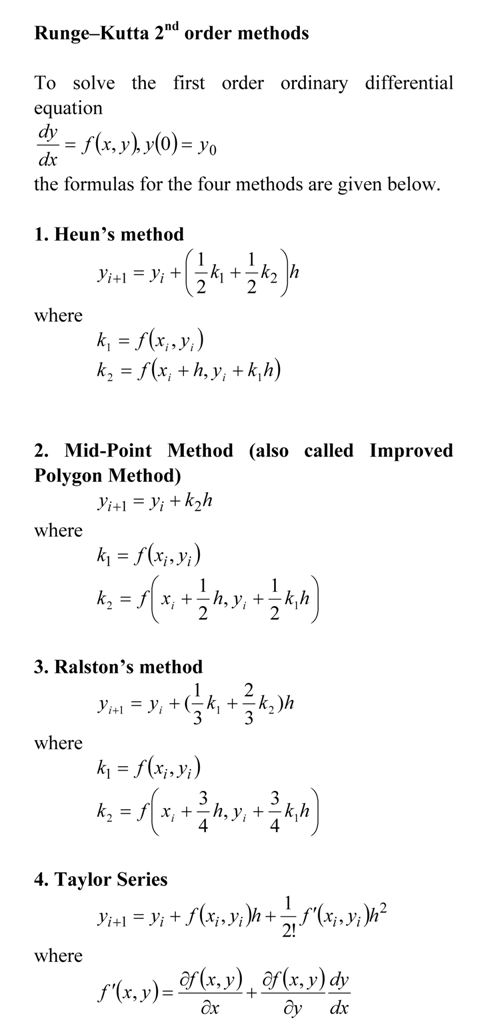
% exact solution to 2nd order Runge-Kutta methods
% of Heun’s method, Ralston’s method, Improved Polygon
% method, and directly using the three terms of Taylor series
clc
clear all
clc
clf
disp(‘This program compares results from the’)
disp(‘exact solution to 2nd order Runge-Kutta methods’)
disp(‘of Heuns method, Ralstons method, Improved Polygon’)
disp(‘ method, and directly using the three terms of Taylor series’)

%INPUTS. If you want to experiment these are only things
% you should and can change. Be sure that the ode has an exact
% solution
% Enter the rhs of the ode of form dy/dx=f(x,y)
fcnstr=’sin(5*x)-0.4*y’ ;
% Initial value of x
x0=0;
% Initial value of y
y0=5;
% Final value of y
xf=5.5;
% number of steps to go from x0 to xf.
% This determines step size h=(xf-x0)/n
n=10;

%REST OF PROGRAM
%Converting the input function to that can be used
f=inline(fcnstr) ;

% EXACT SOLUTION
syms x
eqn=[‘Dy=’ fcnstr]
% exact solution of the ode
exact_solution=dsolve(eqn,’y(0)=5′,’x’)
% geting points for plotting the exact solution
xx=x0:(xf-x0)/100:xf;
yy=subs(exact_solution,x,xx);
yexact=subs(exact_solution,x,xf);
plot(xx,yy,’.’)
hold on

% RUNGE-KUTTA METHODS
h=(xf-x0)/n;
% Heun’s method
a1=0.5;
a2=0.5;
p1=1;
q11=1;
xr=zeros(1,n+1);
yr=zeros(1,n+1);
%Initial values of x and y
xr(1)=x0;
yr(1)=y0;
for i=1:1:n
k1=f(xr(i),yr(i));
k2=f(xr(i)+p1*h,yr(i)+q11*k1*h);
yr(i+1)=yr(i)+(a1*k1+a2*k2)*h;
xr(i+1)=xr(i)+h;
end
%Value of y at x=xf
y_heun=yr(n+1);
% Absolute relative true error for value using Heun’s Method
et_heun=abs((y_heun-yexact)/yexact)*100;
hold on
xlabel(‘x’)
ylabel(‘y’)
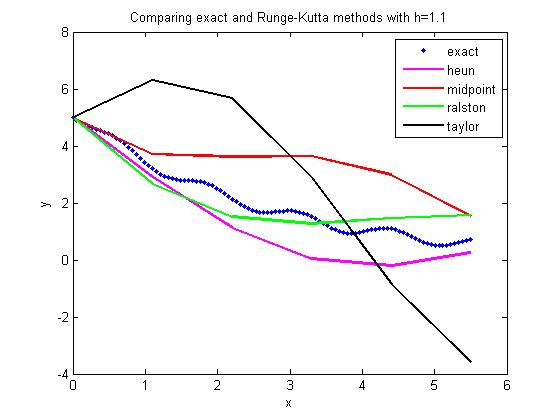
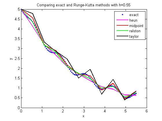
title_name=[‘Comparing exact and Runge-Kutta methods with h=’ num2str(h)] ;
title(title_name)
plot(xr,yr, ‘color’,’magenta’,’LineWidth’,2)
% Midpoint Method (also called Improved Polygon Method)
a1=0;
a2=1;
p1=1/2;
q11=1/2;
%Initial values of x and y
xr(1)=x0;
yr(1)=y0;
for i=1:1:n
k1=f(xr(i),yr(i));
k2=f(xr(i)+p1*h,yr(i)+q11*k1*h);
yr(i+1)=yr(i)+(a1*k1+a2*k2)*h;
xr(i+1)=xr(i)+h;
end
%Value of y at x=xf
y_improved=yr(n+1);
% Absolute relative true error for value using Improved Polygon Method
et_improved=abs((y_improved-yexact)/yexact)*100;
hold on
plot(xr,yr,’color’,’red’,’LineWidth’,2)

% Ralston’s method
a1=1/3;
a2=2/3;
p1=3/4;
q11=3/4;
xr(1)=x0;
yr(1)=y0;
for i=1:1:n
k1=f(xr(i),yr(i));
k2=f(xr(i)+p1*h,yr(i)+q11*k1*h);
yr(i+1)=yr(i)+(a1*k1+a2*k2)*h;
xr(i+1)=xr(i)+h;
end
%Value of y at x=xf
y_ralston=yr(n+1);
% Absolute relative true error for value using Ralston’s Method
et_ralston=abs((y_ralston-yexact)/yexact)*100;
hold on
plot(xr,yr,’color’,’green’,’LineWidth’,2)

% Using first three terms of the Taylor series
syms x y;
fs=char(fcnstr);
% fsp=calculating f'(x,y) using chain rule
fsp=diff(fs,x)+diff(fs,y)*fs;
%Initial values of x and y
xr(1)=x0;
yr(1)=y0;
for i=1:1:n
k1=subs(fs,{x,y},{xr(i),yr(i)});
kk1=subs(fsp,{x,y},{xr(i),yr(i)});
yr(i+1)=yr(i)+k1*h+1/2*kk1*h^2;
xr(i+1)=xr(i)+h;
end
%Value of y at x=xf
y_taylor=yr(n+1);
% Absolute relative true error for value using Taylor series
et_taylor=abs((y_taylor-yexact)/yexact)*100;
hold on
plot(xr,yr,’color’,’black’,’LineWidth’,2)
hold off
legend(‘exact’,’heun’,’midpoint’,’ralston’,’taylor’,1)

% THE OUTPUT
fprintf(‘\nAt x = %g ‘,xf)
disp(‘ ‘)
disp(‘_________________________________________________________________’)
disp(‘Method Value Absolute Relative True Error’)
disp(‘_________________________________________________________________’)
fprintf(‘\nExact Solution %g’,yexact)
fprintf(‘\nHeuns Method %g %g ‘,y_heun,et_heun)
fprintf(‘\nImproved method %g %g ‘,y_improved,et_improved)
fprintf(‘\nRalston method %g %g ‘,y_ralston,et_ralston)
fprintf(‘\nTaylor method %g %g ‘,y_taylor,et_taylor)
disp( ‘ ‘)

________________________________________________________________________________________________

This post is brought to you by Holistic Numerical Methods: Numerical Methods for the STEM undergraduate at http://nm.mathforcollege.com

Subscribe to the blog via a reader or email to stay updated with this blog. Let the information follow you.

Example to show how numerical ODE solutions can be used to find integrals

In a previous post, I enumerated how we can use numerical ODE techniques like Euler and Runge-Kutta methods to find approximate value of definite integrals. Here is an example. Be sure to do the exercises at the end of the post to appreciate the procedure.

_____________________________________________________

This post is brought to you by Holistic Numerical Methods: Numerical Methods for the STEM undergraduate at http://nm.mathforcollege.com

Subscribe to the blog via a reader or email to stay updated with this blog. Let the information follow you.

Comparing Runge-Kutta 2nd order methods

Many a times, students ask me

Which of the Runge-Kutta 2nd order methods gives the most accurate answer to solving a first order ODE?

dy/dx=f(x,y), y(0)=y0

There is no direct answer, although Ralston’s method gives a minimum bound for the truncation error (Ralston, A., Runge-Kutta Methods with Minimum Error Bounds, Match. Compu., Vol 16, page 431, 1962).

They also ask me if using the first three terms of the Taylor series would give a more accurate answer if we calculate $f^{\prime}(x,y)$ symbolically.

The equations for the four methods are given below

Here is the comparison graph for

dy/dx=sin(5*x)-0.4*y, y(0)=5

with

step size of h=1.1

and

step size of h=0.55

This post is brought to you by Holistic Numerical Methods: Numerical Methods for the STEM undergraduate at http://nm.mathforcollege.com

Subscribe to the blog via a reader or email to stay updated with this blog. Let the information follow you.

Can I use numerical solution of ODE techniques to do numerical integration?

Yes.

If you are finding the value of the $latex y=\int_{a}^{b} f(x) dx$, then we can solve the integral as an ordinary differential equation as

dy/dx=f(x), y(a)=0

We can now use any of the numerical techniques such as Euler’s methods and Runge-Kutta methods to find the value of y(b) which would be the approximate value of the integral. Use exact techniques of solving linear ODEs with fixed coefficients such as Laplace transforms, and you can have the exact value of the integral.

_____________________________________________________

This post is brought to you by Holistic Numerical Methods: Numerical Methods for the STEM undergraduate at http://nm.mathforcollege.com

Subscribe to the blog via a reader or email to stay updated with this blog. Let the information follow you.

Time of death – a classic ODE problem

One of the classical applied problems in ordinary differential equations is that of finding the time of death of a homicide victim.

The estimation of time of death is generally based on the temperature of the body at two times – 1) when the victim is found and 2) then a few hours later. Assuming the ambient temperature stays the same and the body is treated as a lumped system, one can use a simple linear ODE to solve the problem.

It is somewhat an inverse problem as we are trying to find the value of the independent variable – the time of death. Here is a solved problem (a pdf version also available).

_____________________________________________________

This post is brought to you by Holistic Numerical Methods: Numerical Methods for the STEM undergraduate at http://nm.mathforcollege.com

Subscribe to the blog via a reader or email to stay updated with this blog. Let the information follow you.