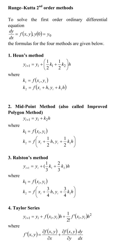
Many a times, students ask me
Which of the Runge-Kutta 2nd order methods gives the most accurate answer to solving a first order ODE?
dy/dx=f(x,y), y(0)=y0
There is no direct answer, although Ralston’s method gives a minimum bound for the truncation error (Ralston, A., Runge-Kutta Methods with Minimum Error Bounds, Match. Compu., Vol 16, page 431, 1962).
They also ask me if using the first three terms of the Taylor series would give a more accurate answer if we calculate f^{\prime}(x,y) symbolically.
The equations for the four methods are given below
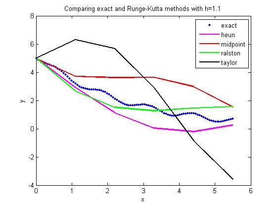
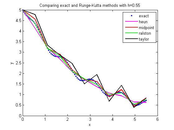
Here is the comparison graph for
dy/dx=sin(5*x)-0.4*y, y(0)=5
with
step size of h=1.1
and
step size of h=0.55
This post is brought to you by Holistic Numerical Methods: Numerical Methods for the STEM undergraduate at http://nm.mathforcollege.com
Subscribe to the blog via a reader or email to stay updated with this blog. Let the information follow you.
I am interested to confirm your several numerical results of this following problem
dy/dx=sin(5*x)-0.4*y, y(0)=5.
I believe that its exact solution can be created easily using symbolic packages. But, because you did not post the answer here, so I try to solve the above first order ODE by alternative method so-called SMT that introduced previously by Denaya Lesa on another topic but also in your numerical blog.
Firstly, write the linear part of the above ODE as following
dyL/dx = -0.4*y , (1)
where its solution is taken in the form
yL = y0*exp(-0.4*x) , with y0=y(0) , (2)
while the nonlinear part as the following
dyN/dx=sin(5*x) , (3)
with the following solution
yN = yN0 + INT05{sin(5*x)}dx , (4)
here, INT05 is integral notation for lower and upper bound of integration 0 and 5 respectively.
Actually yN0 is the integrating constant of the nonlinear part solution. Important to be stressed here, writting in this definite integral only and if only the ODE is solved start from zero value of the independent variable, that is x(0)=0.
In SMT method, every solution of the nonlinear part must be written in a modulation function, that contains an amplitude and a phase function. So, the corresponding of modulation function of eq.(4) is of form
yN = yN0[1 + INT05{sin(5*x)/yN0}dx] , (5)
Finally, the final solution is obtained after substituting yN0 with yL, hence we have
y(x) = 5 exp(-0.4x) +
…. + exp(-0.4x)[INT05{sin(5x)exp(0.4x)}dx] , (6)
In eq.(6) above, I have inserted y0=y(0)=5. Next the problem now reduces to how we can calculate INT05{sin(5x)exp(0.4x)}dx. But I believe this is a simple integral that can be solved analytically.
Dear Mr.Autar Kaw and All,
To complete my explanation of SMT, now I give you all another example of SMT in solving Cauchy Problem :
ty’’ + y’ = -1 , where y’=dy/dt , y(1) = 0, yt’(1) = 0 ,
We know that the commonly way of obtaining its solution is by taking v=y’ , hence the problem reduces to a linear first order ODE tv’ + v = -1.
Now, I focus to give a shortcut solution for the linear first order ODE :
dv/dt + P(t)*v = Q(t) , (1)
Because this linear first order ODE corresponds to the special form of Bernoulli differential equation (BDE) of zero “nonlinearity order (n=0), so we can create its solution from the general solution of BDE.
According to my posting of the BDE’s general solution at the topic Stable Modulation Technique (SMT) previously, for the following BDE :
dv/dt +P(t)*v =Q(t)*v^n , (2) , n is not equal 1.
where I have given the general solution in the following form :
v(t) = exp[-∫P(t)dt]*[ (1-n)∫Q(t)*exp[(1-n)∫P(t)*dt]*dt + C ]^(1/(1-n)) , (3)
here C is integrating constant.
Hence for n = 0, we can take the exact solution of the linear first order ODE in the form :
v(t) = exp[-∫P(t)dt]*[∫Q(t)*exp[∫P(t)dt]*dt + C ] , (4)
It is well known that tv’ + v = -1 can be written as :
v’ + (1/t)*v = -(1/t) , (5)
that corresponds to the variables P(t) = (1/t), and Q(t) = -(1/t). Substituting both variables into eq.(4), we will obtain :
v(t) = exp[-ln(t)]* [INT(-1/t)*exp[ln(t)]*dt + C ] , (6)
After integrating, we have :
v(t) = (1/t) [-t + C1 ] , (7)
Finally by integrating again (v=y’), we obtain :
y(t) = ∫v(t)dt = – t + C1*ln(t) + C2
Okay, next to justify the general solution in eq.(4) for the case of linear first order ODE, now I will create the exact solution by SMT.
Let us consider the SMT’s solving procedure:
Given : dv/dt + P(t)*v = Q(t), (1)
First Step :
Linear part of the DE is of form :
dvL/dt + P(t)*yL = 0, (8)
that gives solution :
vL = CL*exp[-∫P(t)dt] , (9)
here CL is the integrating constant.
Second step : the nonlinear part as :
dvN/dt=Q(t) , (10)
with the solution :
vN = CN + ∫Q(t)dt , (11)
where CN is integrating constant of the nonlinear part.
Next eq.(11) must be written in the following form of a modulation function:
vN = CN*[1 + ∫Q(t)*(1/CN)*dt] , (12)
Third Step :
Replace CN by vL
vN = vL*[1 + ∫Q(t)*(1/vL)*dt] , (13)
After substituting vL of eq.(9) into eq.(13), then we find solution of the linear first order DE in eq.(1) as same as with solution form derived from general solution of Bernoulli equation (n=0),
dv/dt + P(t)*v = Q(t), (1)
that is in the form :
v(t) = exp[-∫P(t)*dt] *[ C + ∫Q(t)*exp[∫P(t)*dt]*dt ] , (14)
where C=CL.
Hopefully, the above explanation can be used as alternative way in solving the Cauchy Problem.
Thank you once again, my best.
Rohedi (http://rohedi.blogspot.com),
Physics Department, Faculty of Mathematics and Natural Sciences,
Sepuluh Nopember Institute of Technology (ITS) Surabaya, Indonesia.
Dear Mr,
I have a problem, how to decide the step size (h) of Runge-kutta scheme when solving an ODE if we don’t know it’s exact solution. For example in solving a special Ricatti differential equation
dy/dt=a(t)y^2 +by+[a(t)]*.
where b is arbitrary constant, and [a(t)]* is the complex conjugate of a(t).
Thank’s for your help.
Nadya Fermega
@Nadya Fermega
I believe the Ricatti differential equation that would be solved is very important for you. But, before performing the accuracy test of Runge kutta scheme to the matlab output, I recommend you to performing the test of numerical scheme in solving the Ricatti differential equation of constant coefficients dy/dx=py^2+qy+r. I ever read it’s general solution that created simplicity using AF(A) diagram in this address
http://eqworld.ipmnet.ru/forum/viewtopic.php?f=2&t=34&start=10. Please visit to site for detail explanation.
Dear All,
The purpose of this post is to annouce a correction for SMT’s procedure for solving the linear first order ODE that posted by me at the first comment here. The correction especially in misstyping the upper of limit integration 5 on the above formulation that to be changed by x variable. Hence, the post is revisited as following.
%%%%%%%%%
I am interested to confirm your several numerical results of this following problem
dy/dx=sin(5*x)-0.4*y, y(0)=5.
I believe that its exact solution can be created easily using symbolic packages. But, because you did not post the answer here, so I try to solve the above first order ODE by alternative method so-called SMT that introduced previously by Denaya Lesa on another topic but also in your numerical blog.
Firstly, write the linear part of the above ODE as following
dyL/dx = -0.4*y , (1)
where its solution is taken in the form
yL = y0*exp(-0.4*x) , with y0=y(0) , (2)
while the nonlinear part as the following
dyN/dx=sin(5*x) , (3)
with the following solution
yN = yN0 + INT0x{sin(5*x)}dx , (4)
here, INT0x is integral notation for lower and upper bound of integration 0 and x respectively.
Actually yN0 is the integrating constant of the nonlinear part solution. Important to be stressed here, writting in this definite integral only and if only the ODE is solved start from zero value of the independent variable, that is x(0)=0.
In SMT method, every solution of the nonlinear part must be written in a modulation function, that contains an amplitude and a phase function. So, the corresponding of modulation function of eq.(4) is of form
yN = yN0[1 + INT0x{sin(5*x)/yN0}dx] , (5)
Finally, the final solution is obtained after substituting yN0 with yL, hence we have
y(x) = 5 exp(-0.4x) +
…. + exp(-0.4x)[INT0x{sin(5x)exp(0.4x)}dx] , (6)
In eq.(6) above, I have inserted y0=y(0)=5. Next the problem now reduces to how we can calculate INT0x{sin(5x)exp(0.4x)}dx. But I believe this is a simple integral that can be solved analytically.
%%%%%%%%%%%
Thank’s for your attention.
Best Regards,
Rohedi.
Hi for All,
Please need help to answer this equation?
What happens with Runge Kutta if you vary the time interval?
Best Wishes
Naji,
Hi for All,
Please need help to answer this equation?
What happens with Runge Kutta if you vary the time interval?
Best Wishes
Naji,
Dear All,
Please need help to answer this equation?
What happens with Runge Kutta if you vary the time interval?
Best Wishes
Naji,
Dear All,
Please need help to answer this equation?
What happens with Runge Kutta if you vary the time interval?
Best Wishes
Naji,
You can change the independent variable as you please but one will need to have some basis for doing so as you do want to write the algorithm in a loop. Adaptive methods used to solve ODEs change the step size based on how the function is behaving.
http://www.tat.physik.uni-tuebingen.de/~speith/Projekt1/numrec/c16-2.pdf
Hi ,
Please i need the confirm the answer for this equation too.
What is the limiting concentration achievable in the still? Demonstrate the answer analytically and using the numerical solution.
Hi ,
Please i need the confirm the answer for this equation too.
What is the limiting concentration achievable in the still? Demonstrate the answer analytically and using the numerical solution.
Hi
Can you help me to solve this equation?
h (d2h/dx2)=4.822h-1.5h3-3.322
Boundary conditions:
X=0 h=0.73
X=-2 dh/dx=0
Regards,
Vahid
Hi
Can you help me to solve this equation?
h (d2h/dx2)=4.822h-1.5h3-3.322
Boundary conditions:
X=0 h=0.73
X=-2 dh/dx=0
Regards,
Vahid