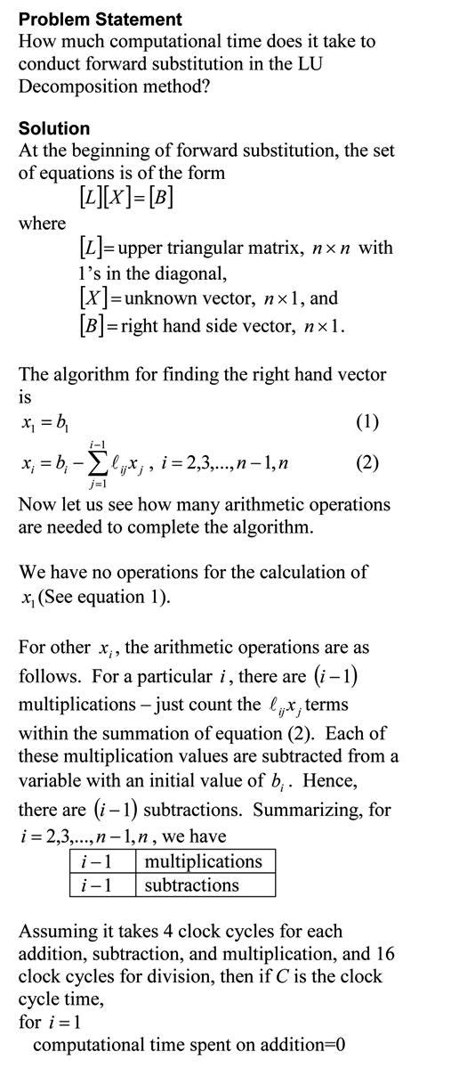
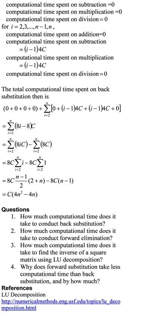
Computational Time for Forward Substitution

In the previous blog, we found the computatational time for back substitution. This is a blog that will show you how we can find the approximate time it takes to conduct forward substitution, while solving simultaneous linear equations. The blog assumes a AMD-K7 2.0GHz chip that uses 4 clock cycles for addition, subtraction and multiplication, while 16 clock cycles for division. Note that we are making reasonable approximations in this blog. Our main motto is to see what the computational time is proportional to – does the computational time double or quadruple if the number of equations is doubled.

Forward Substitution Time

The pdf file of the solution is also available.

This post is brought to you by

Subscribe to the blog via a reader or email to stay updated with this blog. Let the information follow you.

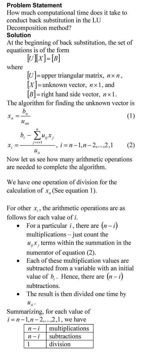
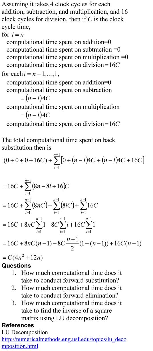
Computational Time for Back Substitution

This is a blog that will show you how we can find the approximate time it takes to conduct back substitution, while solving simultaneous linear equations using Gaussian elimination method. The blog assumes a AMD-K7 2.0GHz chip that uses 4 clock cycles for addition, subtraction and multiplication, and 16 clock cycles for division. Note that we are making reasonable approximations in this blog. Our main motto is to find how the computational time is related to the number of equations.

The pdf file of the solution is also available.

This post is brought to you by

Subscribe to the blog via a reader or email to stay updated with this blog. Let the information follow you.

How do I solve simultaneous linear equations given in equation form?

Many students ask me how do I do this or that in MATLAB.  So I thought why not have a small series of my next few blogs do that.  In this blog, I show you how to solve simultaneous linear equations given in equation form.

  • The MATLAB program link is here.
  • The HTML version of the MATLAB program is here.
  • DO NOT COPY AND PASTE THE PROGRAM BELOW BECAUSE THE SINGLE QUOTES DO NOT TRANSLATE TO THE CORRECT SINGLE QUOTES IN MATLAB EDITOR.  DOWNLOAD THE MATLAB PROGRAM INSTEAD

%% HOW DO I DO THAT IN MATLAB SERIES?
% In this series, I am answering questions that students have asked
% me about MATLAB.  Most of the questions relate to a mathematical
% procedure.

%% TOPIC
% How do I solve a set of simultaneous linear equations
% given in equation form?

%% SUMMARY

% Language : Matlab 2008a;
% Authors : Autar Kaw;
% Mfile available at
% http://nm.mathforcollege.com/blog/sle_equations.m;
% Last Revised : August 22, 2009;
% Abstract: This program shows you how to solve a set of
%     simultaneous linear equations given in equation form?
%           .
clc
clear all
clf

%% INTRODUCTION

disp(‘ABSTRACT’)
disp(‘   This program shows you how to solve a’)
disp(‘   set of simultaneous linear equations given in equation form’)
disp(‘ ‘)
disp(‘AUTHOR’)
disp(‘   Autar K Kaw of http://autarkaw.wordpress.com’)
disp(‘ ‘)
disp(‘MFILE SOURCE’)
disp(‘   http://nm.mathforcollege.com/blog/sle_equations.m’)
disp(‘ ‘)
disp(‘LAST REVISED’)
disp(‘   August 22, 2009’)
disp(‘ ‘)

%% INPUTS
% Enter the equations
eqn1=’12*a+23*b+39*c=29′;
eqn2=’13*a+17*b+19*c=37′;
eqn3=’21*a+23*b+29*c=59’;
%% DISPLAYING INPUTS
disp(‘  ‘)
disp(‘INPUTS’)
disp(‘________________________’)
disp(‘Equations’)
disp(‘________________________’)
disp(eqn1)
disp(eqn2)
disp(eqn3)

%% THE CODE
% The solution
X=solve(eqn1,eqn2,eqn3);
% Assigning the output
a=double(X.a);
b=double(X.b);
c=double(X.c);
%% DISPLAYING OUTPUTS
disp(‘  ‘)
disp(‘OUTPUTS’)
disp(‘________________________’)
disp(‘Solution Vector’)
disp(‘________________________’)
fprintf(‘\nValue of a= %g’,a)
fprintf(‘\nValue of b= %g’,b)
fprintf(‘\nValue of c= %g’,c)
disp(‘  ‘)
disp(‘________________________’)

This post is brought to you by Holistic Numerical Methods: Numerical Methods for the STEM undergraduate at http://nm.mathforcollege.com, the textbook on Numerical Methods with Applications available from the lulu storefront, and the YouTube video lectures available at http://nm.mathforcollege.com/videos and http://www.youtube.com/numericalmethodsguy

Subscribe to the blog via a reader or email to stay updated with this blog. Let the information follow you.

How do I solve a set of simultaneous linear equations given in matrix form?

Many students ask me how do I do this or that in MATLAB.  So I thought why not have a small series of my next few blogs do that.  In this blog, I show you how to solve simultaneous linear equations given in matrix form.

  • The MATLAB program link is here.
  • The HTML version of the MATLAB program is here.
  • DO NOT COPY AND PASTE THE PROGRAM BELOW BECAUSE THE SINGLE QUOTES DO NOT TRANSLATE TO THE CORRECT SINGLE QUOTES IN MATLAB EDITOR.  DOWNLOAD THE MATLAB PROGRAM INSTEAD

%% HOW DO I DO THAT IN MATLAB SERIES?
% In this series, I am answering questions that students have asked
% me about MATLAB.  Most of the questions relate to a mathematical
% procedure.

%% TOPIC
% How do I solve a set of simultaneous linear equations?

%% SUMMARY

% Language : Matlab 2008a;
% Authors : Autar Kaw;
% Mfile available at
% http://nm.mathforcollege.com/blog/sle.m;
% Last Revised : August 12, 2009;
% Abstract: This program shows you how to solve a set of simultaneous linear
% equations?
%           .
clc
clear all
clf

%% INTRODUCTION

disp(‘ABSTRACT’)
disp(‘   This program shows you how to solve a’)
disp(‘   set of simultaneous linear equations’)
disp(‘ ‘)
disp(‘AUTHOR’)
disp(‘   Autar K Kaw of http://autarkaw.wordpress.com’)
disp(‘ ‘)
disp(‘MFILE SOURCE’)
disp(‘   http://nm.mathforcollege.com/blog/sle.m’)
disp(‘ ‘)
disp(‘LAST REVISED’)
disp(‘   August 12, 2009’)
disp(‘ ‘)

%% INPUTS
% Enter the coefficient matrix of the equation [A][X]=[C]
A=[12  23  39; 13  17  19; 21  23  29];
% Enter the right hand side vector
C=[29;   37;  59];
%% DISPLAYING INPUTS
disp(‘  ‘)
disp(‘INPUTS’)
disp(‘________________________’)
disp(‘Coefficient Matrix’)
disp(‘________________________’)
dataval=[A];
disp(dataval)
disp(‘________________________’)
disp(‘Right hand side vector’)
disp(‘________________________’)
dataval=[C];
disp(dataval)
disp(‘________________________’)

%% THE CODE
% The solution
X=A\C;

%% DISPLAYING OUTPUTS
disp(‘  ‘)
disp(‘OUTPUTS’)
disp(‘________________________’)
disp(‘Solution Vector’)
disp(‘________________________’)
dataval=[X];
disp(dataval)
disp(‘________________________’)

his post is brought to you by Holistic Numerical Methods: Numerical Methods for the STEM undergraduate at http://nm.mathforcollege.com, the textbook on Numerical Methods with Applications available from the lulu storefront, and the YouTube video lectures available at http://nm.mathforcollege.com/videos and http://www.youtube.com/numericalmethodsguy

Subscribe to the blog via a reader or email to stay updated with this blog. Let the information follow you.

So what does this mean that the computational time is proportional to some power of n in Gaussian Elimination method?

In a previous post, we talked about why LU Decomposition is computationally more efficient than Gaussian Elimination in some cases. The argument was based on how much computational time does each of the methods take. For example, we said that for back substitution in both methods, the computational time is approximately proportional to $latex n^2/2$.

How did we find that for back substitution the computational time is approximately proportional to $latex n^2/2$?

The amount of time it takes to conduct back substitution depends on the number of floating point operations (FLOPs) needed. Depending on how many FLOPs the computer can execute in a second called FLOPS (note the upper case S to distinguish between FLOPs and FLOPS), that will the determine the actual computational time. (A typical Pentium 4 PC conducts to the order of $latex 10^{9}$ FLOPS; a state-of-art supercomputer conducts to the order of $latex 10^{15}$ FLOPS; in 1983 the PC with a 8087 chip may have conducted to the order of $latex 10^{5}$ FLOPS).

To keep things simple, let’s only count the multiplication/division FLOPs in back substitution as time used by multiplication and division is higher than addition and subtraction (Multiplication may take twice and division as much as thrice the time it takes for addition and subtraction).

In back substitution, we start with the last equation. The last equation involves one division, second last equation involves one multiplication and one division, the third last equation involves two multiplications and one division, and so on. So the number of multiplication/divisions FLOPs is 1 for last equation, 2 for second last equation, 3 for third last equation, that is, for all equations, $latex 1+2….+n=n^2/2+n/2 $. For large n, this number is approximately $latex n^2/2$.

This post brought to you by Holistic Numerical Methods: Numerical Methods for the STEM undergraduate at http://nm.mathforcollege.com

Rusty on Matrix Algebra

Eight years ago, the Florida legislature decided to reduce the number of credit hours it takes a state university student to graduate with an undergrad engineering degree. The number of credit hours were reduced from 136 to 128. One of the courses that got the ax in the Mechanical Engineering Department at USF was a 2-credit hour Linear Algebra course. There are many other universities in the nation that have done the same.

So how do students learn Linear Algebra when the course is one of the requirements for accreditation of engineering programs?

Some universities have bundled Linear Algebra course content into courses such as Quantitative Methods where students are expected, in many cases, to learn linear algebra, a programming language/computational system, and complex analysis. Other curriculums have dispersed the Linear Algebra content into different courses such as the topic of special matrices in Programming, simultaneous linear equations in Statics, and eigenvalues/eigenvectors in Vibrations, etc. Unless quality controls are introduced carefully, the content/depth of Linear Algbera in such courses can vary substantially between courses and instructors. Such control is impossible in metropolitan universities such as USF where a large proportion of students transfer from community colleges.

To have a resource that would be a self-explanatory as well as get the students exposed to Linear Algebra applications motivated me to write a simple Introduction to Matrix Algebra book. The book consists of ten chapters spanning fundamentals of matrix algebra, numerical methods for solving a set of equations, and a treatment of adequacy of solutions and eigenvalues.

Since 2002, the Introduction to Matrix Algebra book has been downloaded free of charge by more than 30,000 users from 50 different countries, and the feedback has been humbling and fulfilling.

Since April 2008, the book has also been made available for a nominal charge via lulu.com as a pdf file as well as a soft cover book. Proceeds from the book are allowing me to expand the book with more examples/problems and additional chapters.

Since my belief continues to embrace open and uncomplicated dissemination, eight individual chapters of the book in pdf form are still available free of charge. So one may ask the following question. Why should I buy the book when it is available free of charge? For answer to this question, click here

For more details about the book, visit the book website at http://autarkaw.com/books/matrixalgebra/index.html

This post brought to you by Holistic Numerical Methods: Numerical Methods for the STEM undergraduate at http://nm.mathforcollege.com
LU Decomposition takes more computational time than Gaussian Elimination! What gives?

If you are solving a set of simultaneous linear equations, LU Decomposition method (involving forward elimination, forward substitution and back substitution) would use more computational time than Gaussian elimination (involving forward elimination and back substitution, but NO forward substitution).

So why use and waste time talking about LU Decomposition?

Because, LU Decomposition is computationally more efficient than Gaussian elimination when we are solving several sets of equations with the same coefficient matrix but different right hand sides. Case in point is when you are finding the inverse of a matrix [A]. If one is trying to find the inverse of nxn matrix, then it implies that one needs to solve n sets of simultaneous linear equations of [A][X]=[C] form with the n right hand sides [C] being the n columns of the nxn identity matrix, while the coefficient matrix [A] stays the same.

The computational time taken for solving a single set of n simultaneous linear equations is as follows:

  • Forward elimination: Proportional to \frac{n^3}{3}
  • Back substitution: Proportional to \frac{n^2}{2}
  • Forward substitution: Proportional to \frac{n^2}{2}

So for LU decomposition method used to find the inverse of a matrix, the computational time is proportional to \frac{n^3}{3}+n( \frac{n^2}{2}+\frac{n^2}{2})=\frac{4n^3}{3}. Remember that the forward elimination only needs to be done only once on [A] to generate the L and U matrices for the LU decomposition method. However the forward and back substitution need to be done n times.

Now for Gaussian Elimination used to find the inverse of a matrix, the computational time is proportional to n \frac{n^3}{3} +n \frac{n^2}{2}=\frac{n^4}{3}+\frac{n^3}{2}. Remember that both the forward elimination and back substitution need to be done n times.

Hence for large n, for LU Decomposition, the computational time is proportional to \frac{4n^3}{3}, while for Gaussian Elimination, the computational time is proportional to \frac{n^4}{3} . So for large n, the ratio of the computational time for Gaussian elimination to computational for LU Decomposition is {\frac{n^4}{3}}/{\frac{4n^3}{3}}=\frac{n}{4}

As an example, to find the inverse of a 2000×2000 coefficient matrix by Gaussian Elimination would take n/4=2000/4=500 times the time it would take to find the inverse by LU Decomposition.

So are you convinced now why we use LU Decomposition in certain cases? For textbook notes on this issue, examples of LU Decomposition to solve a set of equations, and finding inverse of a matrix using LU Decomposition, click here.

Reference: Numerical Methods for the STEM Undergraduate, http://nm.mathforcollege.com/topics/lu_decomposition.html

This post brought to you by Holistic Numerical Methods: Numerical Methods for the STEM undergraduate at http://nm.mathforcollege.com