Misconceptions about diagonal and tridiagonal matrices

A reader wrote: “I purchased on lulu the 2nd edition of your Introduction to Matrix Algebra for self study, and the book just arrived. I started reading it and found some annoying errors. For example on Chapter 1, page 5: for the first (diagonal) matrix, why is there a zero located in a33, when you defined on the previous page that only diagonal entries of square matrix can be non-zero (this answer is different on your free online pdf) . Also, on page 6 for the tridiagonal matrix, why is there a zero located in the diagonal below the major diagonal? I was wondering if you can provide me with the list of errors and corrections, because it’s going to be very difficult to study the material on my own and the errors in the book just makes it more frustrating.”

My answer: “There is no erratum issued yet on the book.

A diagonal matrix is diagonal based on the nondiagonal elements being zero. The diagonal elements have no restrictions. They can be zero or nonzero.

A tridiagonal matrix is a square matrix in which all elements not on the following are zero – the major diagonal, the above the major diagonal, and the diagonal below the major diagonal. The major diagonal, the diagonal above the major diagonal, and the diagonal below the major diagonal have no restrictions. They can be zero or nonzero.

The concerns you have raised are some of the common misconceptions students develop about these special matrices.

______________________________________________

This post is brought to you by Holistic Numerical Methods: Numerical Methods for the STEM undergraduate at http://nm.MathForCollege.com, the textbook on Numerical Methods with Applications available from the lulu storefront, the textbook on Introduction to Programming Concepts Using MATLAB, and the YouTube video lectures available at http://nm.MathForCollege.com/videos. Subscribe to the blog via a reader or email to stay updated with this blog. Let the information follow you.
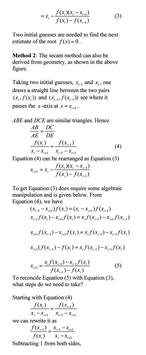
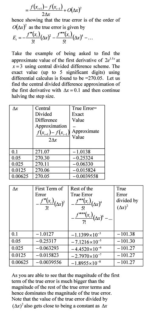
Making sense of the Big Oh!

Many students are challenged to understand the nature of Big Oh in relating it to the order of accuracy of numerical methods.  In this exercise, we are using the central divided difference approximation of the first derivative of the function to ease some of the mystery surrounding the Big Oh.


You can visit the above example by opening a pdf file.

This post is brought to you by Holistic Numerical Methods: Numerical Methods for the STEM undergraduate at http://nm.MathForCollege.com, the textbook on Numerical Methods with Applications available from the lulu storefront, the textbook on Introduction to Programming Concepts Using MATLAB, and the YouTube video lectures available at http://nm.MathForCollege.com/videos.  Subscribe to the blog via a reader or email to stay updated with this blog. Let the information follow you.
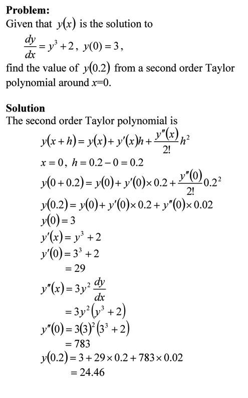
Using Taylor polynomial to approximately solve an ordinary differential equation

Taylor polynomial is an essential concept in understanding numerical methods. Examples abound and include finding accuracy of divided difference approximation of derivatives and forming the basis for Romberg method of numerical integration.

In this example, we are given an ordinary differential equation and we use the Taylor polynomial to approximately solve the ODE for the value of the dependent variable at a particular value of the independent variable. As a homework assignment, do the following.
1) compare the approximate solution with the exact one, and
2) get another approximate solution by using a third order Taylor polynomial.

Taylor polynomial approximation of solving ordinary differential equations

You can visit the above example by opening a pdf or video file.

This post is brought to you by Holistic Numerical Methods: Numerical Methods for the STEM undergraduate at http://nm.MathForCollege.com, the textbook on Numerical Methods with Applications available from the lulu storefront, the textbook on Introduction to Programming Concepts Using MATLAB, and the YouTube video lectures available at http://nm.MathForCollege.com/videos.  Subscribe to the blog via a reader or email to stay updated with this blog. Let the information follow you.

2012 in review

The WordPress.com stats helper monkeys prepared a 2012 annual report for this blog.

Here’s an excerpt:

19,000 people fit into the new Barclays Center to see Jay-Z perform. This blog was viewed about 150,000 times in 2012. If it were a concert at the Barclays Center, it would take about 8 sold-out performances for that many people to see it.

Click here to see the complete report.

Proving the denominator of the linear regression formula for its constants is greater than zero.

In a previous blog, we wrote without proof that the denominator of the constants of the linear regression formulas are greater than zero.  In this blog, we show the proof.


This post is brought to you by Holistic Numerical Methods: Numerical Methods for the STEM undergraduate at http://nm.mathforcollege.com, the textbook on Numerical Methods with Applications available from the lulu storefront, the textbook on Introduction to Programming Concepts Using MATLAB, and the YouTube video lectures available athttp://nm.mathforcollege.com/videos.  Subscribe to the blog via areader or email to stay updated with this blog. Let the information follow you.

Prove that the least squares general straight-line model gives the absolute minimum of the sum of the squares of the residuals?

Many regression models when derived in books only show the first derivative test to find the formulas for the constants of a linear regression model.  Here we show a thoroughly explained derivation.


___________________________________________

This post is brought to you by Holistic Numerical Methods: Numerical Methods for the STEM undergraduate at http://nm.mathforcollege.com, the textbook on Numerical Methods with Applications available from the lulu storefront, the textbook on Introduction to Programming Concepts Using MATLAB, and the YouTube video lectures available at http://nm.mathforcollege.com/videos.  Subscribe to the blog via a reader or email to stay updated with this blog. Let the information follow you.
Effect of Significant Digits: Example 2: Regression Formatting in Excel

In a series of bringing pragmatic examples of the effect of significant digits, we discuss the influence of using default and scientific formats in the trendline function of Microsoft Excel.  This is the second example (first example was on a beam deflection problem) in the series.

____________________________________________

This post is brought to you by Holistic Numerical Methods: Numerical Methods for the STEM undergraduate at http://nm.mathforcollege.com, the textbook on Numerical Methods with Applications available from the lulu storefront, the textbook on Introduction to Programming Concepts Using MATLAB, and the YouTube video lectures available at http://nm.mathforcollege.com/videos.  Subscribe to the blog via a reader or email to stay updated with this blog. Let the information follow you.
Effect of Significant Digits: Example 1: Beam Deflection

In a series of bringing pragmatic examples of the effect of significant digits, we discuss the exact solution of finding the deflection in a simply supported beam with a uniform load and a tensile axial load.

___________________________________________

This post is brought to you by Holistic Numerical Methods: Numerical Methods for the STEM undergraduate at http://nm.mathforcollege.com, the textbook on Numerical Methods with Applications available from the lulu storefront, the textbook on Introduction to Programming Concepts Using MATLAB, and the YouTube video lectures available at http://nm.mathforcollege.com/videos.  Subscribe to the blog via a reader or email to stay updated with this blog. Let the information follow you.
Length of curve

This is a solution to the problem I gave to the class in a recent test.

A robot follows a path generated by a quadratic interpolant from x=2 to x=4.  The interpolant passes through three consecutive data points (2,4), (3,9) and (4,16) and is given by y=x2.  Find the best estimate of the length of the interpolant path from x=2 to x=4. 

The solution is given as an audio pdf (also called pencast – need Adobe X reader or higher). Three methods are shown. I expected one to use Method 2 or Method 3.
http://www.eng.usf.edu/~kaw/class/EML3041/livescribe/length_of_curve.pdf

______________________________________________________________

This post is brought to you by Holistic Numerical Methods: Numerical Methods for the STEM undergraduate at http://nm.mathforcollege.com, the textbook on Numerical Methods with Applications available from the lulu storefront, the textbook on Introduction to Programming Concepts Using MATLAB, and the YouTube video lectures available at http://nm.mathforcollege.com/videos.  Subscribe to the blog via a reader or email to stay updated with this blog. Let the information follow you.
Example: How many significant digits are correct in my answer?

In the previous post I showed you the theorem that tells us how many significant digits are correct in our numerical solution that is iterative in nature.  In this post, we illustrate this with an example.

__________________________________________
This post is brought to you by Holistic Numerical Methods: Numerical Methods for the STEM undergraduate at http://nm.mathforcollege.com, the textbook on Numerical Methods with Applications available from the lulu storefront, the textbook on Introduction to Programming Concepts Using MATLAB, and the YouTube video lectures available at http://nm.mathforcollege.com/videos.  Subscribe to the blog via a reader or email to stay updated with this blog. Let the information follow you.