Ian Sanders and Autar Kaw
As we are back in face-to-face classes, we may wish to again conduct multiple-choice question examinations in the classroom without the use of computers to alleviate academic integrity concerns, not have to depend on the reliability of the laptop battery and available WiFi, and not have to continue to make different tests every semester.
Background
Commercially available OMR (optical mark recognition) exam sheets, scanners, and processing software can cost educators and educational institutions thousands of dollars per year. In response to this, OpenMCR has been developed as a free and easy-to-use alternative. The tool includes a multiple-choice exam sheet and works with any scanner and printer.
Here are the steps to use the program.
Step 1: Print out the MCQ sheets
Depending on the number of questions being asked, whether it is less than 75 or more (the maximum number of questions that can be asked is 150), you will first choose one of the two pdf files to print.
-
-
-
- 75 Question Variant (Download the pdf file from here)
- 150 Question Variant (Download the pdf file from here)
Step 2: Download the program to your PC
Go here https://github.com/iansan5653/open-mcr/releases and download the open-mcr.zip file that is available under assets. Extract the zip file to the directory of your choice. One of the files you will see amongst the extracted files is open-mcr.exe. That is the one you need to double-click on to run the program.
For more details about this open resource software, go to https://github.com/iansan5653/open-mcr
Step 3: Choose your variant of the key
In addition to reading scanned images, the software can also automatically score exam results. It does this by comparing the provided keys with the output. There are three options for this, depending on which way you generate your exams:
1. One Exam Variant
This is the most common exam variant. If you give every exam-taker the exact same exam, you can instruct them to leave the Test Form Code field blank on their sheets. In addition, leave that field blank on the answer key sheet. All exam results will be compared to the single answer key sheet provided. Skip to Step 4 if this is what you chose – no need to create confusion.
2. Shuffled Exam Variants
If you provide the exam-takers with multiple variants of the same exam, and these variants differ only in question order (in other words, each variant is simply shuffled), then you can score all of these with the same key file by providing a file that defines the orders of the shuffled variants.
Each row in this file represents a key, and each column represents the position that that question should be moved to.
For example, if the exam form A has questions 1, 2, and 3, the exam form B might have them in 3, 1, 2 order and C might have them in 3, 2, 1 order. This would result in the following arrangement file:
Test Form Code, Q1, Q2, Q3
             A,  1,  2,  3
             B,  3,  1,  2
             C,  3,  2,  1
If this were the file you upload, then all of the exams with form A would be left untouched while B and C would be rearranged to 1, 2, 3 order. Select the file in the program under the Select Form Arrangement Map.
Note that the first row in this file should always be in 1, 2, 3, … order, and each row after that should only have one instance of each number.
If you use this option, only one exam key can be provided or an error will be raised.
3. Distinct Exam Variants
Finally, you can provide the exam-takers with multiple wholly distinct variants of the same exam. In this case, each exam will be scored by selecting the answer key with an exactly matching Test Form Code. No rearrangement will be performed.
Step 4: Conduct the test
Give the question paper and the blank MCQ sheet to the students. Ask them to bubble items such as last name, first name, middle name, student id, course number, key code, and their answer responses.
Step 5: Scan the MCQ sheets and the key(s)
If you would like to take advantage of the automatic grading feature of the software, you must provide it with one or more answer keys. To create an answer key, simply print a normal sheet and put 9999999999 in the Student ID field. Also, add a Test Form Code which will be used to match students’ exams with the correct answer key, and finally, fill in the exam with the correct answers.
This is optional – you can choose to just have the software read the exams and not score them.
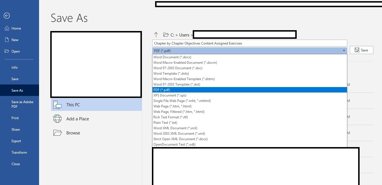
Scan all the student and key MCQ sheets on a copier or a scanner into a single PDF file. Use Adobe Acrobat DC or any other freely available program to export the pdf file to images.
Step 6: Run the program
One of the files you will see amongst the extracted files from Step 2 is open-mcr.exe. That is the one you need to double-click on to run the program.
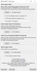
Select the input folder where the images of the MCQ sheets are.
If you select the convert multiple answers in a question to ‘F’ option, then if a student selects, for example, A and B for a question, the output file will save that as F instead of [A|B].
If you select the save empty in questions as ‘G’ option, if a student skips a question by leaving it blank, the output file will save that as G instead of as a blank cell.
Choose the proper Form Variant as 75 Questions or 150 questions.
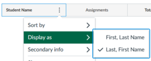
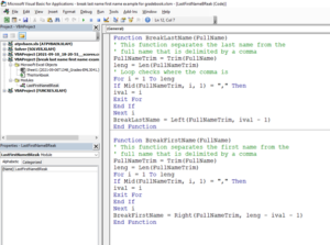
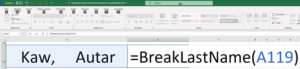
Under Select Output Folder, click Browse, and select the folder where you would like to save the resulting CSV files. If you select the sort results by name option, results will be sorted by the students’ last, first, and middle names (in that order). Otherwise, results will be saved in the order they were processed.
Press Continue and watch the progress of the program.
Step 7: Output Files
After the program finishes processing, results will be saved as CSV files in your selected output folder. These files can be opened in Excel or in any text editor. Files will be saved with the time of processing to avoid overwriting any existing files.
If you did not include any answer keys, one raw file will be saved with all of the students’ selected answers, and no scoring is performed.
If you did include one or more answer keys, two more files will be saved in addition to the aforementioned raw file. One of these files will have all of the keys that were found, and the other will have the scored results. In the scored file, questions are saved for each student as either 1 (correct) or 0 (incorrect).
Software License
Copyright (C) 2019-22 Ian Sanders
This program is free software: you can redistribute it and/or modify it under the terms of the GNU General Public License as published by the Free Software Foundation, either version 3 of the License, or (at your option) any later version.
This program is distributed in the hope that it will be useful, but WITHOUT ANY WARRANTY; without even the implied warranty of MERCHANTABILITY or FITNESS FOR A PARTICULAR PURPOSE. See the GNU General Public License for more details.
For the full license text, see license.txt.
Multiple-Choice Sheet License
The multiple-choice sheet distributed with this software is licensed under the Creative Commons Attribution-NonCommercial-ShareAlike 4.0 International license (CC BY-NC-SA 4.0). In summary, this means that you are free to distribute and modify the document so long as you share it under the same license, provide attribution, and do not use it for commercial purposes. For the full license, see the Creative Commons website.
Note: You are explicitly allowed to distribute the multiple-choice sheet without attribution if using it unmodified for educational purposes and not in any way implying that it is your own work. This is an exception to the Creative Commons terms.