Taylor series example

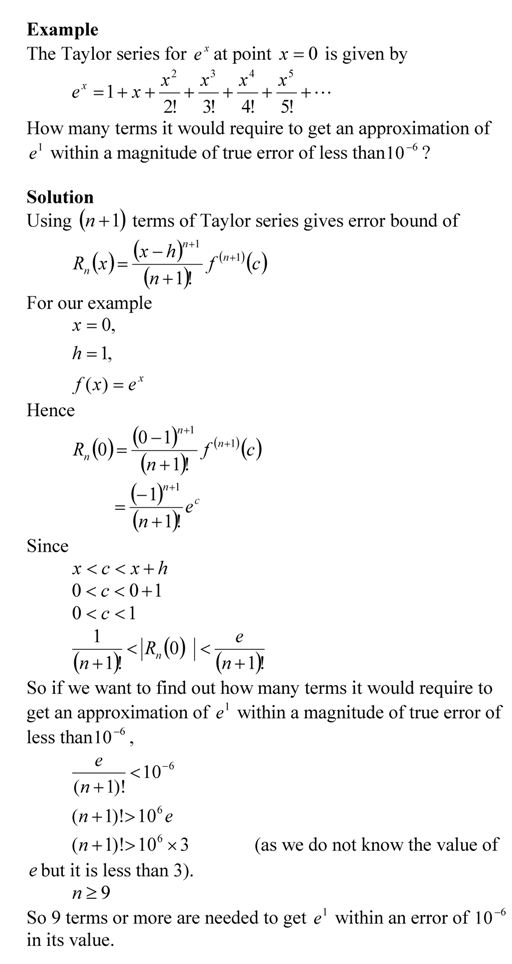
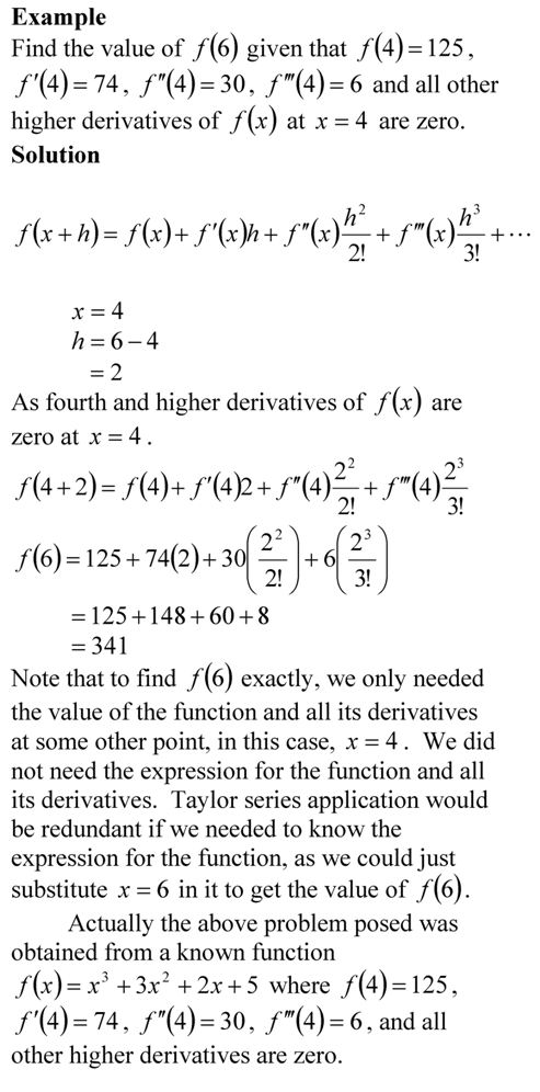
If Archimedes were to quote Taylor’s theorem, he would have said, “Give me the value of the function  and the value of all (first, second, and so on) its derivatives at a single point, and I can give you the value of the function at any other point”.

It is very important to note that the Taylor’s theorem is not asking for the expression of the function and its derivatives, just the value of the function and its derivatives at a single point.

Now the fine print: Yes, all the derivatives have to exist and be continuous between x and x+h, the point where you are wanting to calculate the function at. However, if you want to calculate the function approximately by using the nth order Taylor polynomial, then 1st, 2nd,…., nth derivatives need to exist and be continuous in the closed interval [x,x+h], while the (n+1)th derivative needs to exist and be continuous in the open interval (x,x+h).

Taylor Series Revisited

Taylor series is a very important concept that is used in numerical methods. From the concept of truncation error to finding the true error in Trapezoidal rule, having a clear understanding of Taylor series is extremely important. Other places in numerical methods where Taylor series concept is used include: the derivation of finite difference formulas for derivatives, finite difference method of solving differential equations, error in Newton Raphson method of solving nonlinear equations, Newton divided difference polynomial for interpolation, etc.

I have written a short chapter on Taylor series. After reading the chapter, you should be able to:

1. understand the basics of Taylor’s theorem,

2. see how transcendental and trigonometric functions can be written as Taylor’s polynomial,

3. use Taylor’s theorem to find the values of a function at any point, given the values of the function and all its derivatives at a particular point,

4. errors and error bounds of approximating a function by Taylor series,

5. revisit the chapter whenever Taylor’s theorem is used to derive or explain numerical methods for various mathematical procedures.

This post is brought to you by Holistic Numerical Methods: Numerical Methods for the STEM undergraduate at http://nm.mathforcollege.com.

An abridged (for low cost) book on Numerical Methods with Applications will be in print (includes problem sets, TOC, index) on December 10, 2008 and available at lulu storefront.

Subscribe to the blog via a reader or email to stay updated with this blog. Let the information follow you.
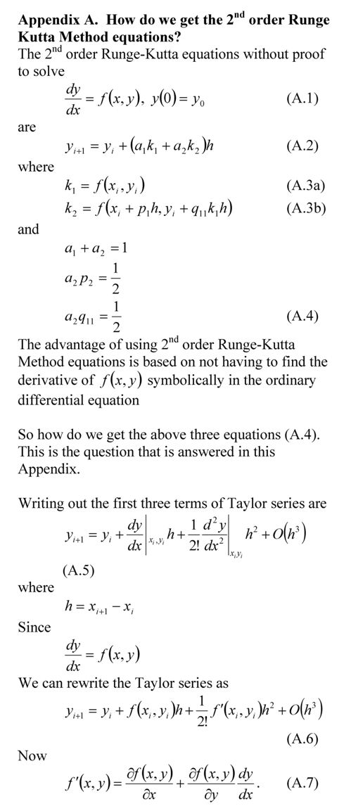
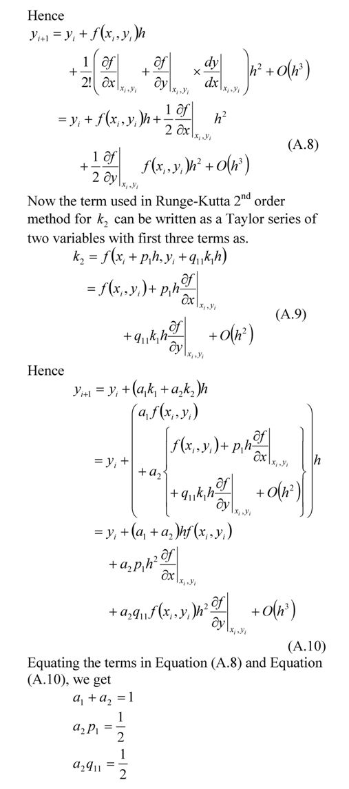
Runge-Kutta 2nd order equations derived

In my class, I present the 2nd order Runge-Kutta method equations without proof. Although I do discuss where the equations come from, there are still students who want to see the proof. So here it is.

_____________________________________________________

This post is brought to you by Holistic Numerical Methods: Numerical Methods for the STEM undergraduate at http://nm.mathforcollege.com

Subscribe to the blog via a reader or email to stay updated with this blog. Let the information follow you.
A Matlab program for comparing Runge-Kutta methods

In a previous post, we compared the results from various 2nd order Runge-Kutta methods to solve a first order ordinary differential equation. In this post, I am posting the matlab program. It is better to download the program as single quotes in the pasted version do not translate properly when pasted into a mfile editor of MATLAB or see the html version for clarity and sample output .

Do your own testing on a different ODE, a different value of step size, a different initial condition, etc. See the inputs section below that is colored in bold brick.

% Simulation : Comparing the Runge Kutta 2nd order method of
% solving ODEs
% Language : Matlab 2007a
% Authors : Autar Kaw
% Last Revised : July 12, 2008
% Abstract: This program compares results from the
% exact solution to 2nd order Runge-Kutta methods
% of Heun’s method, Ralston’s method, Improved Polygon
% method, and directly using the three terms of Taylor series
clc
clear all
clc
clf
disp(‘This program compares results from the’)
disp(‘exact solution to 2nd order Runge-Kutta methods’)
disp(‘of Heuns method, Ralstons method, Improved Polygon’)
disp(‘ method, and directly using the three terms of Taylor series’)

%INPUTS. If you want to experiment these are only things
% you should and can change. Be sure that the ode has an exact
% solution
% Enter the rhs of the ode of form dy/dx=f(x,y)
fcnstr=’sin(5*x)-0.4*y’ ;
% Initial value of x
x0=0;
% Initial value of y
y0=5;
% Final value of y
xf=5.5;
% number of steps to go from x0 to xf.
% This determines step size h=(xf-x0)/n
n=10;


%REST OF PROGRAM
%Converting the input function to that can be used
f=inline(fcnstr) ;

% EXACT SOLUTION
syms x
eqn=[‘Dy=’ fcnstr]
% exact solution of the ode
exact_solution=dsolve(eqn,’y(0)=5′,’x’)
% geting points for plotting the exact solution
xx=x0:(xf-x0)/100:xf;
yy=subs(exact_solution,x,xx);
yexact=subs(exact_solution,x,xf);
plot(xx,yy,’.’)
hold on

% RUNGE-KUTTA METHODS
h=(xf-x0)/n;
% Heun’s method
a1=0.5;
a2=0.5;
p1=1;
q11=1;
xr=zeros(1,n+1);
yr=zeros(1,n+1);
%Initial values of x and y
xr(1)=x0;
yr(1)=y0;
for i=1:1:n
k1=f(xr(i),yr(i));
k2=f(xr(i)+p1*h,yr(i)+q11*k1*h);
yr(i+1)=yr(i)+(a1*k1+a2*k2)*h;
xr(i+1)=xr(i)+h;
end
%Value of y at x=xf
y_heun=yr(n+1);
% Absolute relative true error for value using Heun’s Method
et_heun=abs((y_heun-yexact)/yexact)*100;
hold on
xlabel(‘x’)
ylabel(‘y’)
title_name=[‘Comparing exact and Runge-Kutta methods with h=’ num2str(h)] ;
title(title_name)
plot(xr,yr, ‘color’,’magenta’,’LineWidth’,2)
% Midpoint Method (also called Improved Polygon Method)
a1=0;
a2=1;
p1=1/2;
q11=1/2;
%Initial values of x and y
xr(1)=x0;
yr(1)=y0;
for i=1:1:n
k1=f(xr(i),yr(i));
k2=f(xr(i)+p1*h,yr(i)+q11*k1*h);
yr(i+1)=yr(i)+(a1*k1+a2*k2)*h;
xr(i+1)=xr(i)+h;
end
%Value of y at x=xf
y_improved=yr(n+1);
% Absolute relative true error for value using Improved Polygon Method
et_improved=abs((y_improved-yexact)/yexact)*100;
hold on
plot(xr,yr,’color’,’red’,’LineWidth’,2)

% Ralston’s method
a1=1/3;
a2=2/3;
p1=3/4;
q11=3/4;
xr(1)=x0;
yr(1)=y0;
for i=1:1:n
k1=f(xr(i),yr(i));
k2=f(xr(i)+p1*h,yr(i)+q11*k1*h);
yr(i+1)=yr(i)+(a1*k1+a2*k2)*h;
xr(i+1)=xr(i)+h;
end
%Value of y at x=xf
y_ralston=yr(n+1);
% Absolute relative true error for value using Ralston’s Method
et_ralston=abs((y_ralston-yexact)/yexact)*100;
hold on
plot(xr,yr,’color’,’green’,’LineWidth’,2)

% Using first three terms of the Taylor series
syms x y;
fs=char(fcnstr);
% fsp=calculating f'(x,y) using chain rule
fsp=diff(fs,x)+diff(fs,y)*fs;
%Initial values of x and y
xr(1)=x0;
yr(1)=y0;
for i=1:1:n
k1=subs(fs,{x,y},{xr(i),yr(i)});
kk1=subs(fsp,{x,y},{xr(i),yr(i)});
yr(i+1)=yr(i)+k1*h+1/2*kk1*h^2;
xr(i+1)=xr(i)+h;
end
%Value of y at x=xf
y_taylor=yr(n+1);
% Absolute relative true error for value using Taylor series
et_taylor=abs((y_taylor-yexact)/yexact)*100;
hold on
plot(xr,yr,’color’,’black’,’LineWidth’,2)
hold off
legend(‘exact’,’heun’,’midpoint’,’ralston’,’taylor’,1)

% THE OUTPUT
fprintf(‘\nAt x = %g ‘,xf)
disp(‘ ‘)
disp(‘_________________________________________________________________’)
disp(‘Method Value Absolute Relative True Error’)
disp(‘_________________________________________________________________’)
fprintf(‘\nExact Solution %g’,yexact)
fprintf(‘\nHeuns Method %g %g ‘,y_heun,et_heun)
fprintf(‘\nImproved method %g %g ‘,y_improved,et_improved)
fprintf(‘\nRalston method %g %g ‘,y_ralston,et_ralston)
fprintf(‘\nTaylor method %g %g ‘,y_taylor,et_taylor)
disp( ‘ ‘)

________________________________________________________________________________________________

This post is brought to you by Holistic Numerical Methods: Numerical Methods for the STEM undergraduate at http://nm.mathforcollege.com

Subscribe to the blog via a reader or email to stay updated with this blog. Let the information follow you.
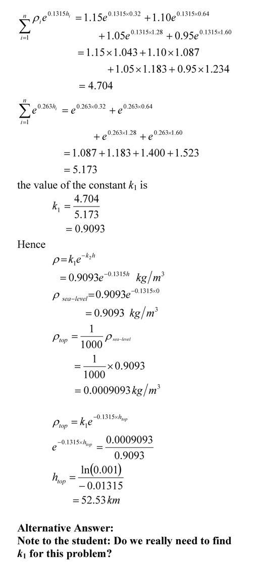
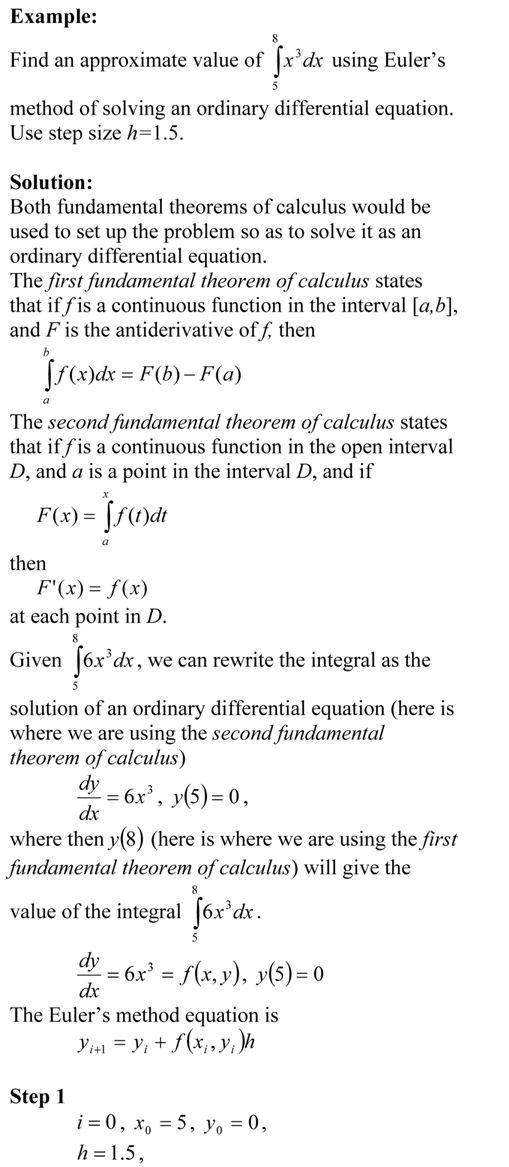
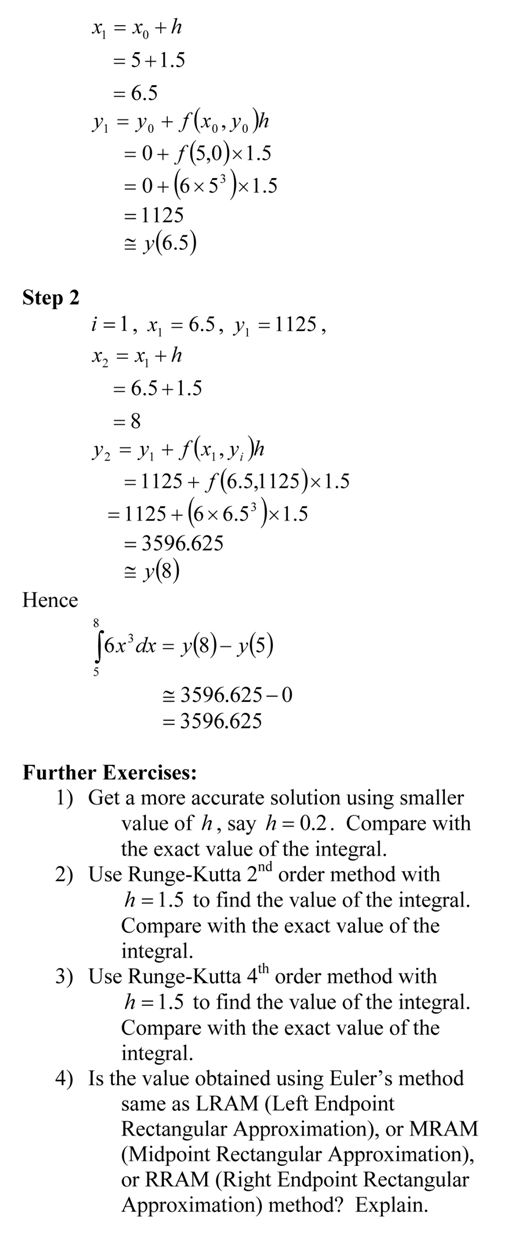
Example to show how numerical ODE solutions can be used to find integrals

In a previous post, I enumerated how we can use numerical ODE techniques like Euler and Runge-Kutta methods to find approximate value of definite integrals. Here is an example. Be sure to do the exercises at the end of the post to appreciate the procedure.

_____________________________________________________

This post is brought to you by Holistic Numerical Methods: Numerical Methods for the STEM undergraduate at http://nm.mathforcollege.com

Subscribe to the blog via a reader or email to stay updated with this blog. Let the information follow you.
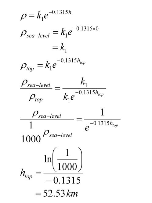
Comparing Runge-Kutta 2nd order methods

Many a times, students ask me

Which of the Runge-Kutta 2nd order methods gives the most accurate answer to solving a first order ODE?

dy/dx=f(x,y), y(0)=y0

There is no direct answer, although Ralston’s method gives a minimum bound for the truncation error (Ralston, A., Runge-Kutta Methods with Minimum Error Bounds, Match. Compu., Vol 16, page 431, 1962).

They also ask me if using the first three terms of the Taylor series would give a more accurate answer if we calculate f^{\prime}(x,y) symbolically.

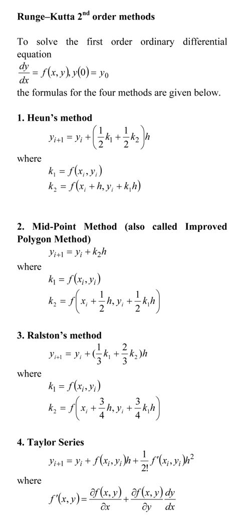
The equations for the four methods are given below

Here is the comparison graph for

dy/dx=sin(5*x)-0.4*y, y(0)=5

with

step size of h=1.1

and

step size of h=0.55

This post is brought to you by Holistic Numerical Methods: Numerical Methods for the STEM undergraduate at http://nm.mathforcollege.com

Subscribe to the blog via a reader or email to stay updated with this blog. Let the information follow you.
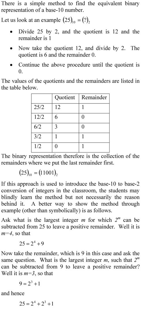
Can I use numerical solution of ODE techniques to do numerical integration?

Yes.

If you are finding the value of the $latex y=\int_{a}^{b} f(x) dx$, then we can solve the integral as an ordinary differential equation as

dy/dx=f(x), y(a)=0

We can now use any of the numerical techniques such as Euler’s methods and Runge-Kutta methods to find the value of y(b) which would be the approximate value of the integral. Use exact techniques of solving linear ODEs with fixed coefficients such as Laplace transforms, and you can have the exact value of the integral.

_____________________________________________________

This post is brought to you by Holistic Numerical Methods: Numerical Methods for the STEM undergraduate at http://nm.mathforcollege.com

Subscribe to the blog via a reader or email to stay updated with this blog. Let the information follow you.
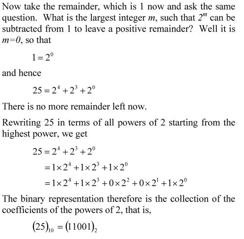
Time of death – a classic ODE problem

One of the classical applied problems in ordinary differential equations is that of finding the time of death of a homicide victim.

The estimation of time of death is generally based on the temperature of the body at two times – 1) when the victim is found and 2) then a few hours later. Assuming the ambient temperature stays the same and the body is treated as a lumped system, one can use a simple linear ODE to solve the problem.

It is somewhat an inverse problem as we are trying to find the value of the independent variable – the time of death. Here is a solved problem (a pdf version also available).

_____________________________________________________

This post is brought to you by Holistic Numerical Methods: Numerical Methods for the STEM undergraduate at http://nm.mathforcollege.com

Subscribe to the blog via a reader or email to stay updated with this blog. Let the information follow you.
Is it just a coincidence – true error in multiple segment Trapezoidal rule gets approximately quartered as the number of segments is doubled?

Look at the table below. This is a table that shows the approximate value of the integral

$latex \int_{8}^{30} 2000 ln \frac{140000}{140000-2100t}-9.8t dt $

as a function of the number of segments used in the Trapezoidal rule and the corresponding true error.

n

Value

Et

1

11868

-807

2

11266

-205

3

11153

-91.4

4

11113

-51.5

5

11094

-33.0

6

11084

-22.9

7

11078

-16.8

8

11074

-12.9

The true error for n=1 is -807 and for n=2 is -205. As you can see the quarter of -807 is approximately -201.75 and close to the true error for n=2. Is this a coincidence?

Look at the true error for n=2 which is -205 and for n=4 is -51.5. As you can see the quarter of -205 is approximately -51.75 and close to the value of the true error for n=4. Is this a coincidence?

No. This is because the true error in a single segment trapezoidal rule is

$latex \frac{(b-a)^3}{12} f^{\prime\prime} (c)$

where c is some point not known but in the domain [a,b] of $latex \int_{a}^{b} f(x) dx$. It can be then shown (see page 14 of this pdf file for full proof) that for the multiple segment trapezoidal rule, the true error is

$latex \frac{(b-a)^3}{12n^2} f^{\prime\prime} $

where the $latex f^{\prime\prime}$ is an average value of the second derivative of the function f(x) calculated at some point within each of the n segments. Since a and b are constant, and $latex f^{\prime\prime}$ becomes almost a constant as n increases, the true error is approximately inversely proportional to the square of the number of segments.

Note to the reader: Develop a similar table as given above for an integral of your choice and see it for yourself if the true error gets approximately quartered as the number of segments is doubled.

_____________________________________________________

This post is brought to you by Holistic Numerical Methods: Numerical Methods for the STEM undergraduate at http://nm.mathforcollege.com

Subscribe to the blog via a reader or email to stay updated with this blog. Let the information follow you.
Can I use Trapezoidal rule to calculate an improper integral?

For example, $latex \int_{a}^{infinity} e^{-x} dx $ is an improper integral which can be calculated exactly as $latex e^{-a}$.

Can we solve this integral by multiple segment Trapezoidal rule when we already know that the upper limit is infinity?

Yes, we can solve it in spite of the upper limit being infinity. We first need to make a change of variables such as $latex t=\frac{1}{x}$, then $latex dx=-\frac{1}{t^2}dt$ giving $latex \int_{1/a}^{0} e^{-1/t} (-1/t^2) dt $

But even for this integral we have issues as the integrand gives division by zero problems at t=0 (although the limit itself is zero at t=0).

The MATLAB program that can be downloaded at http://nm.mathforcollege.com/blog/trapezoidal_improper.m (better to download it as the single quotes do not translate well with matlab editor) shows that we get accurate results for transformed integral with 256 segments.
% Simulation : Can I use Trapezoidal rule for an improper integral?
% Language : Matlab 2007a
% Authors : Autar Kaw, http://nm.mathforcollege.com
% mfile available at
% http://nm.mathforcollege.com/blog/trapezoidal_improper.m
% Last Revised : July 15, 2008
% Abstract: This program shows use of multiple segment Trapezoidal
% rule to integrate exp(-x) from x=a to infinity, where a>0.
clc
clear all
disp(‘This program shows the convergence of getting the value of ‘)
disp(‘an improper integral using multiple segment Trapezoidal rule’)
disp(‘Author: Autar K Kaw. autarkaw.wordpress.com’)

%INPUTS. If you want to experiment, these are the only variables
% you should and can change.
% a = Lower limit of integration
a=1/2;

fprintf(‘\nFinding the integral of exp(-x) from a to infinity where a=%g’,a)

% SIMULATION
syms x
% integrand exp(-x)
f=exp(-x);
valexact=double(int(f,x,a,inf));
fprintf(‘\n\nExact value of integral = %f’,valexact)
disp( ‘ ‘)

% Transformed integrand by change of variables
ft=inline(‘exp(-1/t)*(-1/t^2)’);
% Limits of integration
at=1/a;
b=0;

%finding value of the integral using 16, 32, 64, 128 and 256 segments
for k=4:1:8
n=2^k;
h=(b-at)/n;
sum=0;
for i=1:1:n-1
sum=sum+ft(at+i*h);
end
% See how f(b) is not added as f(b)=infinity. But
% using a different value of the function at one point or
% finite number of points does not change the value of the
% integral. We are substituting f(b)=0
sum=2*sum+ft(at)+0;
sum=(b-at)/(2*n)*sum;
fprintf(‘\nApproximate value of integral =%f with %g segments’,sum,n)
end
disp(‘ ‘)
This program shows the convergence of getting the value of
an improper integral using multiple segment Trapezoidal rule
Author: Autar K Kaw. autarkaw.wordpress.com

Finding the integral of exp(-x) from a to infinity where a=0.5

Exact value of integral = 0.606531

Approximate value of integral =0.605971 with 16 segments
Approximate value of integral =0.606496 with 32 segments
Approximate value of integral =0.606521 with 64 segments
Approximate value of integral =0.606528 with 128 segments
Approximate value of integral =0.606530 with 256 segments

Published with MATLAB® 7.3

Now someone may rightly point out that it works well because the limit of the integrand is zero at the lower limit of integration for the above mentioned integral.

So go ahead, modify the program for doing this improper integral $latex \int_{0}^{4} \frac{1}{\sqrt {x}} dx $ and see how well it works. In this case the integrand is singular at $latex x=0$ and one would have to assume the function to be a number other than infinity at $latex x=0$ for applying the multiple segment Trapezoidal rule.

How many segments do you need to get an accurate answer for this integral?

_____________________________________________________

This post is brought to you by Holistic Numerical Methods: Numerical Methods for the STEM undergraduate at http://nm.mathforcollege.com

Subscribe to the blog via a reader or email to stay updated with this blog. Let the information follow you.