Uncategorized – Page 6 – Numerical Methods Guy

A simple MATLAB program to show that High order interpolation is a bad idea

In a previous post, we talked about that higher order interpolation is a bad idea.

Runge's function

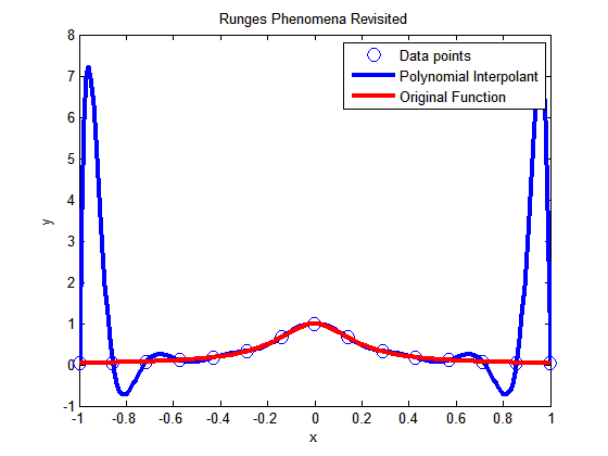
In this post I am showing you a MATLAB program that will allow you to experiment by changing the number of data points you choose, that is, the value of n (see the input highlighted in red in the code – this is the only line you want to change) and see for yourself why high order interpolation is a bad idea. Just, cut and paste the code below (or download it from http://www.eng.usf.edu/~kaw/download/runge.m) in the MATLAB editor and run it.

% Simulation : Higher Order Interpolation is a Bad Idea

% Language : Matlab r12
% Authors : Autar Kaw
% Last Revised : June 10 2008
% Abstract: In 1901, Carl Runge published his work on dangers of high order
% interpolation. He took a simple looking function f(x)=1/(1+25x^2) on
% the interval [-1,1]. He took points equidistantly spaced in [-1,1]
% and interpolated the points with polynomials. He found that as he
% took more points, the polynomials and the original curve differed
% even more considerably. Try n=5 and n=25
clc
clear all
clf

disp(‘In 1901, Carl Runge published his work on dangers of high order’)
disp(‘interpolation. He took a simple looking function f(x)=1/(1+25x^2) on’)
disp(‘the interval [-1,1]. He took points equidistantly spaced in [-1,1]’)
disp(‘and interpolated the points with a polynomial. He found that as he’)
disp(‘took more points, the polynomials and the original curve differed’)
disp(‘even more considerably. Try n=5 and n=15’)

%
% INPUT:
% Enter the following
% n= number of equidisant x points from -1 to +1
n=15;

% SOLUTION
disp(‘ ‘)
disp(‘SOLUTION’)
disp(‘Check out the plots to appreciate: High order interpolation is a bad idea’)
fprintf(‘\nNumber of data points used =%g’,n)
% h = equidisant spacing between points
h=2.0/(n-1);
syms xx
% generating n data points equally spaced along the x-axis
% First data point
x(1)=-1;
y(1)=subs(1/(1+25*xx^2),xx,-1);
% Other data points
for i=2:1:n
x(i)=x(i-1)+h;
y(i)=subs(1/(1+25*xx^2),xx,x(i));
end

% Generating the (n-1)th order polynomial from the n data points
p=polyfit(x,y,n-1);

% Generating the points on the polynomial for plotting
xpoly=-1:0.01:1;
ypoly=polyval(p,xpoly);

% Generating the points on the function itself for plotting
xfun=-1:0.01:1;
yfun=subs(1/(1+25*xx^2),xx,xfun);

% The classic plot
% Plotting the points
plot(x,y,’o’,’MarkerSize’,10)
hold on
% Plotting the polynomial curve
plot(xpoly,ypoly,’LineWidth’,3,’Color’,’Blue’)
hold on
% Plotting the origianl function
plot(xfun,yfun,’LineWidth’,3,’Color’,’Red’)
hold off
xlabel(‘x’)
ylabel(‘y’)
title(‘Runges Phenomena Revisited’)
legend(‘Data points’,’Polynomial Interpolant’,’Original Function’)
%***********************************************************************
disp(‘ ‘)
disp(‘ ‘)
disp(‘What you will find is that the polynomials diverge for’)
disp(‘0.726<|x|<1. If you started to choose same number of points ‘)
disp(‘but more of them close to -1 and +1, you would avoid such divergence. ‘)
disp(‘ ‘)
disp(‘However, there is no general rule to pick points for a general ‘)
disp(‘function so that this divergence is avoided; but some rules do exist for ‘)
disp(‘certian types of functions.’)

This post is brought to you by Holistic Numerical Methods: Numerical Methods for the STEM undergraduate at http://nm.mathforcollege.com

High order interpolation is a bad idea?

One would intuitively assume that if one was given 100 data points of data, it would be most accurate to interpolate the 100 data points to a 99th order polynomial. More the merrier: is that not the motto. But I am sorry to burst your bubble – high order interpolation is generally a bad idea.

The classic example (dating as back as 1901 before there were calculators) to show that higher order interpolation idea is a bad idea comes from the famous German mathematician Carl Runge.

He took a simple and smooth function, f(x) = 1/(1+25x^2) in the domain [-1,1]. He chose equidisant x-data points on the function f(x) in the domain xε[-1,1]. Then he used those data points to draw a polynomial interpolant.

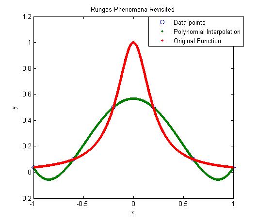
For example, if I chose 6 data points equidistantly spaced on [-1,1], those are (-1, 0.038462), (-0.6, 0.1), (-0.2,0.5), (0.2,0.5), (0.6,0.1), and (1,0.038462). I can interpolate these 6 data points by a 5th order polynomial. In Figure 1, I am then plotting the fifth order polynomial and the original function. You can observe that there is a large difference between the original function and the polynomial interpolant. The polynomial does go through the six points, but at many other points it does not even come close to the original function. Just look at x= 0.85, the value of the function is 0.052459, but the fifth order polynomial gives you a value of -0.055762, a whopping 206.30 % error; also note the opposite sign.

Figure 1. 5th order polynomial interpolation with six equidistant points.

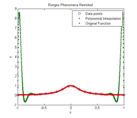
Maybe I am not taking enough data points. Six points may be too small a number to approximate the function. Ok! Let’s get crazy. How about 20 points? That will give us a 19th order polynomial. I will choose 20 points equidistantly in [-1,1].

Figure 2. 19th order polynomial interpolation with twenty equidistant points

It is not any better though it did do a better job of approximating the function except near the ends. At the ends, it is worse than before. At our chosen point, x= 0.85, the value of the function is 0.052459, while we get -0.62944 from the 19th order polynomial, and that is a big whopper error of 1299.9 %.

So are you convinced that higher order interpolation is a bad idea? Try an example by yourself: step function y=-1, -1<x<0 and y=+1, 0<x<1.

What is the alternative to higher order interpolation? Is it lower order interpolation, but does that not use data only from less points than are given. How can we use lower order polynomials and at the same time use information from all the given data points. The answer to that question is SPLINE interpolation.

This post is brought to you by Holistic Numerical Methods: Numerical Methods for the STEM undergraduate at http://nm.mathforcollege.com

If a polynomial of order n or less passes thru (n+1) points, it is unique!

Given n+1 (x,y) data pairs, with all x values being unique, then a polynomial of order n or less passes thru the (n+1) data points. How can we prove that this polynomial is unique?

I am going to show you the proof for a particular case and you can extend it to polynomials of any order n.

Lets suppose you are given three data points (x1,y1), (x2,y2), (x3,y3) where x1 $\ne$ x2 $\ne$ x3.

Then if a polynomial P(x) of order 2 or less passes thru the three data points, we want to show that P(x) is unique.

We will prove this by contradiction.

Let there be another polynomial Q(x) of order 2 or less that goes thru the three data points. Then R(x)=P(x)-Q(x) is another polynomial of order 2 or less. But the value of P(x) and Q(x) is same at the three x-values of the data points x1, x2, x3. Hence R(x) has three zeros, at x=x1, x2 and x3.

But a second order polynomial only has two zeros; the only case where a second order polynomial can have three zeros is if R(x) is identically equal to zero, and hence have infinite zeros. Since R(x)=P(x)-Q(x), and R(x) $\equiv$ 0, then P(x) $\equiv$ Q(x). End of proof.

But how do you know that a second order polynomial with three zeros is identically zero.

R(x) is of the form a0+a1*x+a2*x^2 and has three zeros, x1, x2, x3. Then it needs to satisfy the following three equations

a0+a1*x1+a2*x1^2=0

a0+a1*x2+a2*x2^2=0

a0+a1*x3+a2*x3^2=0

The above equations have the trivial solution a0=a1=a2=0 as the only solution if

det(1 x1 x1^2; 1 x2 x2^2; 1 x3 x3^2) $\ne$ 0.

That is in fact the case as

det(1 x1 x1^2; 1 x2 x2^2; 1 x3 x3^2) = (x1-x2)*(x2-x3)*(x3-x1),

and since x1 $\ne$ x2 $\ne$ x3, the

det(1 x1 x1^2; 1 x2 x2^2; 1 x3 x3^2) $\ne$ 0

So the only solution is a0=a1=a2=0 making R(x) $\equiv$ 0

This post brought to you by Holistic Numerical Methods: Numerical Methods for the STEM undergraduate at http://nm.mathforcollege.com

An experiment to illustrate numerical differentiation, integration, regression and ODEs

Aluminum Cylinder Dipped in Iced Water Starting Summer 2007, five experiments have been introduced in the course in Numerical Methods at USF. I will discuss each experiment in a separate blog as the

summer trods along.

Experiment#1: Cooling an aluminum cylinder

The first experiment illustrates use of numerical differentiation, numerical integration, regression and ordinary differential equations. In this experiment, an aluminum cylinder is immersed in a bath of iced water. As you can see in the figure, two thermocouples are attached to the cylinder and are connected to a temperature indicator. Readings of temperature as a function of time are taken in intervals of 5 seconds for a total of 40 seconds. The temperature of the iced-water bath is also noted.

If you just want the data for a typical experiment conducted in class, click here and here for data.

The students are now assigned about 10 problems to do. These include

finding the convection coefficient (involves nonlinear regression – it is also a good example of where the data for a nonlinear model does not need to be transformed to use linear regression)
finding the rate of change of temperature to calculate rate at which is heat is stored in the cylinder (involves numerical differentiation)
prediction of temperatures from solution of ordinary differential equations
finding reduction in the diameter of the aluminum cylinder (involves numerical integration as the thermal expansion coefficient is a function of temperature)

This post brought to you by Holistic Numerical Methods: Numerical Methods for the STEM undergraduate at http://nm.mathforcollege.com

Rusty on Matrix Algebra

Eight years ago, the Florida legislature decided to reduce the number of credit hours it takes a state university student to graduate with an undergrad engineering degree. The number of credit hours were reduced from 136 to 128. One of the courses that got the ax in the Mechanical Engineering Department at USF was a 2-credit hour Linear Algebra course. There are many other universities in the nation that have done the same.

So how do students learn Linear Algebra when the course is one of the requirements for accreditation of engineering programs?

Some universities have bundled Linear Algebra course content into courses such as Quantitative Methods where students are expected, in many cases, to learn linear algebra, a programming language/computational system, and complex analysis. Other curriculums have dispersed the Linear Algebra content into different courses such as the topic of special matrices in Programming, simultaneous linear equations in Statics, and eigenvalues/eigenvectors in Vibrations, etc. Unless quality controls are introduced carefully, the content/depth of Linear Algbera in such courses can vary substantially between courses and instructors. Such control is impossible in metropolitan universities such as USF where a large proportion of students transfer from community colleges.

To have a resource that would be a self-explanatory as well as get the students exposed to Linear Algebra applications motivated me to write a simple Introduction to Matrix Algebra book. The book consists of ten chapters spanning fundamentals of matrix algebra, numerical methods for solving a set of equations, and a treatment of adequacy of solutions and eigenvalues.

Since 2002, the Introduction to Matrix Algebra book has been downloaded free of charge by more than 30,000 users from 50 different countries, and the feedback has been humbling and fulfilling.

Since April 2008, the book has also been made available for a nominal charge via lulu.com as a pdf file as well as a soft cover book. Proceeds from the book are allowing me to expand the book with more examples/problems and additional chapters.

Since my belief continues to embrace open and uncomplicated dissemination, eight individual chapters of the book in pdf form are still available free of charge. So one may ask the following question. Why should I buy the book when it is available free of charge? For answer to this question, click here

For more details about the book, visit the book website at http://autarkaw.com/books/matrixalgebra/index.html

This post brought to you by Holistic Numerical Methods: Numerical Methods for the STEM undergraduate at http://nm.mathforcollege.com

Round off errors and the Patriot missile

Twenty-eight Americans were killed on February 25, 1991 when an Iraqi Scud hit the Army barracks in Dhahran, Saudi Arabia. The Patriot defense system had failed to track and intercept the Scud. What was the cause for this failure?

The Patriot defense system consists of an electronic detection device called the range gate. It calculates the area in the air space where it should look for the target such as a Scud. To find out where the Patriot missile should be next, it calculates its location based on the velocity of the Scud and the last time the radar detected the Scud.

In the Patriot missile, time was saved in a fixed point register that had a length of 24 bits. Since the internal clock of the system is measured every one-tenth of a second, 1/10 expressed in a 24 bit fixed point register is 0.0001100110011001100110011 (the exact value of the representation 0.0001100110011001100110011 of 1/10 in the 24-fixed point register is 209715/2097152) . As we can see that this is not an exact representation of 1/10. It would take infinite numbers of bits to represent 1/10 exactly. So, the error in the representation is (1/10-209715/2097152) which is approximately 9.5E-8 seconds.

On the day of the mishap, the battery on the Patriot missile was left on for 100 consecutive hours, hence causing an inaccuracy of 9.5E-8x10x60x60x100=0.34 seconds (10 clock cycles in a second, 60 seconds in a minute, 60 minutes in an hour).

The shift calculated in the range gate due to the error of 0.342 seconds was calculated as 687m. For the Patriot missile defense system, the target is considered out of range if the shift is more than than 137m. The shift of larger than 137m resulted in the Scud not being targeted and hence killing 28 Americans in the barracks of Saudi Arabia. Scud-B missile

When I started looking at the Google search results of the problem, I found some very useful resources that would be of interest to the reader. These go beyond the above given simplistic explanation of the problem and tell the story behind the story. Here they are

This reference is the full GAO report of the investigation that resulted after the accident. “Patriot Missile Defense – Software Problem Led to System Failure at Dhahran, Saudi Arabia”, GAO Report, General Accounting Office, Washington DC, February 4, 1992.
It should be pointed out that the Patriot missile was originally designed to be a mobile system and not used as a anti-ballistic system. In mobile systems, the clocks are reset more often. As per the article Operations: I Did Not Say You Could Do That! by Bill Barnes and Duke McMillin, here are some important observations: “It turns out that the original use case for this system was to be mobile and to defend against aircraft that move much more slowly than ballistic missiles. Because the system was intended to be mobile, it was expected that the computer would be periodically rebooted. In this way, any clock-drift error would not be propagated over extended periods and would not cause significant errors in range calculation. Because the Patriot system was not intended to run for extended times, it was probably never tested under those conditions—explaining why the problem was not discovered until the war was in progress. The fact that the system was also designed as an antiaircraft system probably also enabled the inclusion of such a design flaw, because slower-moving airplanes would be easier to track and, therefore, less dependent upon a highly accurate clock value.”

A student asked me why we did not use a clock cycle that could be represented exactly in the 24 bit register. Close to 1/10 is a number 0.125 that can be represented exactly as 0.001000000000000000000000 in a 24-bit register, and where 8 clock cycles would be equal to 1 second. I do not have an answer to this question but I intend to find out from my computer science colleagues.

This post brought to you by Holistic Numerical Methods: Numerical Methods for the STEM undergraduate at http://nm.mathforcollege.com

Undergraduate Numerical Methods for Engineering

I am starting this blog to help UNDERGRADUATES with their queries on Numerical Methods for Engineers. I have been teaching Numerical Methods for the last 20 years and I get interesting queries and questions while I am teaching, when students come to see me during my office hours, or the email sent at midnight before the assignment is due.

I am keeping a log of what students ask me and will note the answers to their queries here. I am sure that students elsewhere have similar questions when they take a course in Numerical Methods.

The diversity of the course is quite evident –

The course is taught to different engineering majors – mechanical, civil, chemical, industrial and electrical.
Some teachers emphasize the numerical methods while others spend more time on solving physical problems, and a few may include numerical analysis.
The programming tools are diverse including FORTRAN (yes the language is alive and well), Basic, C, Java, or computational packages such as MATLAB, MATHEMATICA, MathCAD, and Maple.

With funding from NSF since 2002, we have developed web-based resources for a course in Numerical Methods. The inclusion of the blog is not part of the funded proposals but we think that this mode of Web 2.0 dissemination is critical in keeping the conversation going on. Although what I am doing here can be offered via a static website, the widgets offered by blogging softwares are indispensable. The widgets I like are categorizing, tagging and RSS Feeds.

We want to reach as many people as possible and build a community which may be temporary to students who are taking a course in Numerical Methods, permanent to instructors and people who use numerical methods in their work. But one thing is certain, temporary or permanent, visitors will leave their imprint on this resource.

This post brought to you by Holistic Numerical Methods: Numerical Methods for the STEM undergraduate at http://nm.mathforcollege.com