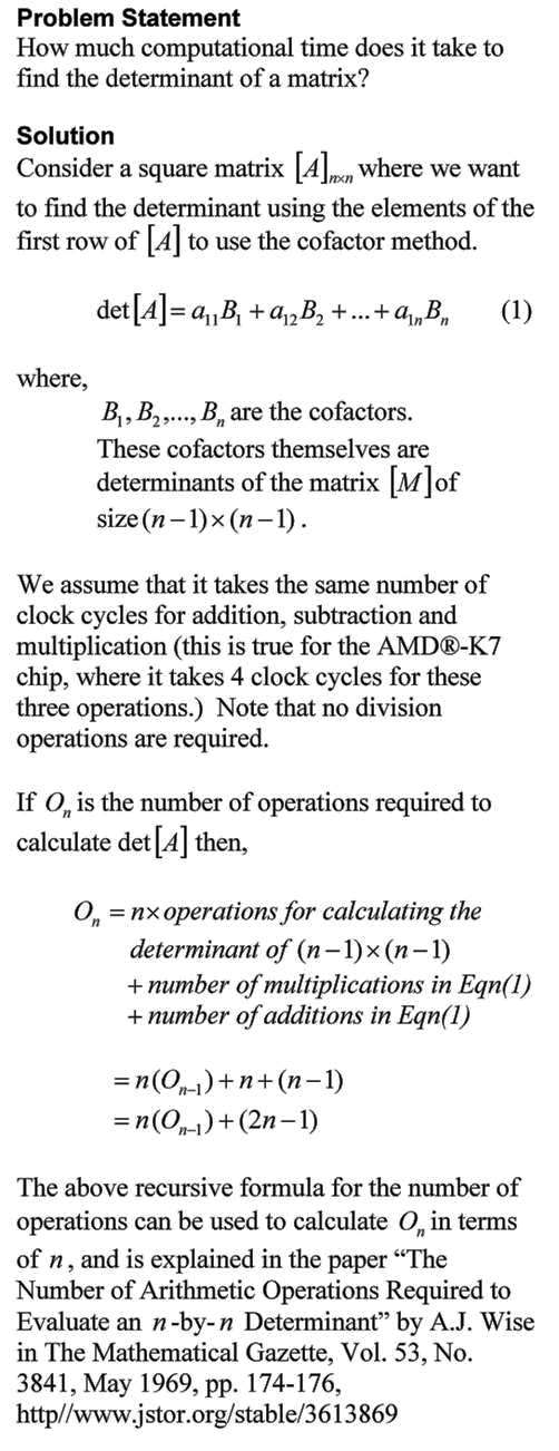
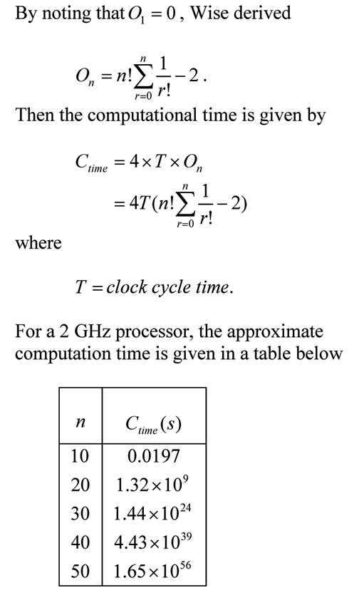
A Wolfram demo on converting a decimal number to floating point binary representation

Here is another Wolfram demo. This one converts a decimal number to a floating point binary representation.  To play with the demo, download the free CDF player first.
 
The total number of bits used for the representation =
       one bit for the sign of the number +
       one bit for the sign of the exponent +
       number of bits for the exponent +
       number of bits for the mantissa +
       As an example, how would 54.75 be represented in a 9-bit register where the first bit is used for the sign of the number, second bit is used for sign of exponent, next three bits are used for the exponent, and the last four bits are used for the mantissa?
Both the number and the exponent are positive. 
As the number is normalized to lie between 1 and 2 (the interval being half-closed at the bottom and half-open at the top), the leading binary digit is always 1. So we do not actually use it in the representation of the mantissa. Hence the mantissa bits are 1011. Moreover the exponent bits are 101, the sign of the number bit is 0, and the sign of the exponent bit is 0.
Therefore the representation is .
 

Reference: Floating Point Representation

This post is brought to you by

Holistic Numerical Methods: Numerical Methods for the STEM undergraduate at http://nm.mathforcollege.com, the textbook on Numerical Methods with Applications available from the lulu storefront, the textbook on Introduction to Programming Concepts Using MATLAB, and the YouTube video lectures available at http://nm.mathforcollege.com/videos.  Subscribe to the blog via a reader or email to stay updated with this blog. Let the information follow you.

A Wolfram Demo for Numerical Differentiation

We are in the process of developing Wolfram Demonstrations for Numerical Methods.  In this demo, we show approximations of derivatives by finite difference formulas.  We compare three difference approximations with the exact value.  To play with the demo, download the free CDF player first.


Reference: Approximation of First Derivatives by Finite Difference Approximations

This post is brought to you by

Subscribe to the blog via a reader or email to stay updated with this blog. Let the information follow you.

Taylor Series in Layman’s terms

The Taylor series for a function f(x) of one variable x is given by
f(x+h) = f(x) + f '(x)h +f ''(x) h^2/2!+ f ''' (x)h^3/3! + .............

What does this mean in plain English?
As Archimedes would have said (without the fine print), “Give me the value of the function at a single point, and the value of all (first, second, and so on) its derivatives, and I can give you the value of the function at any other point”.
It is very important to note that the Taylor series is not asking for the expression of the function and its derivatives, just the value of the function and its derivatives at a single point.

Now the fine print: Yes, all the derivatives have to exist and be continuous between x (the point where you are) to the point, x+h where you are wanting to calculate the function at. However, if you want to calculate the function approximately by using the n^{th} order Taylor polynomial, then 1^{st}, 2^{nd} ……., n^{th} derivatives need to exist and be continuous in the closed interval [x, x+h] , while the n+1^{th} derivative needs to exist and be continuous in the open interval (x, x+h).

Reference: Taylor Series Revisited

This post is brought to you by

Subscribe to the blog via a reader or email to stay updated with this blog. Let the information follow you.

Computational Time for Forward Substitution

In the previous blog, we found the computatational time for back substitution. This is a blog that will show you how we can find the approximate time it takes to conduct forward substitution, while solving simultaneous linear equations. The blog assumes a AMD-K7 2.0GHz chip that uses 4 clock cycles for addition, subtraction and multiplication, while 16 clock cycles for division. Note that we are making reasonable approximations in this blog. Our main motto is to see what the computational time is proportional to – does the computational time double or quadruple if the number of equations is doubled.

Forward Substitution Time

The pdf file of the solution is also available.

This post is brought to you by

Subscribe to the blog via a reader or email to stay updated with this blog. Let the information follow you.

Computational Time for Back Substitution

This is a blog that will show you how we can find the approximate time it takes to conduct back substitution, while solving simultaneous linear equations using Gaussian elimination method. The blog assumes a AMD-K7 2.0GHz chip that uses 4 clock cycles for addition, subtraction and multiplication, and 16 clock cycles for division. Note that we are making reasonable approximations in this blog. Our main motto is to find how the computational time is related to the number of equations.

The pdf file of the solution is also available.

This post is brought to you by

Subscribe to the blog via a reader or email to stay updated with this blog. Let the information follow you.

Taylor Series Exercise – Method 3

Taylor series is an important concept for learning numerical methods – not only for understanding how trigonometric and transcendental functions are calculated by a computer, but also for error analysis in numerical methods. I asked the question below in the first test in the course, and half of the students did not get to the final answer. In a previous blog, I showed you the method that most instructors would use. See how some students approached (another approach) the problem.

Taylor Series Exercise Method 3

The pdf file of the solution is also available.

This post is brought to you by

Subscribe to the blog via a reader or email to stay updated with this blog. Let the information follow you.

Taylor Series Exercise – Method 2

Taylor series is an important concept for learning numerical methods – not only for understanding how trigonometric and transcendental functions are calculated by a computer, but also for error analysis in numerical methods. I asked the question below in the first test in the course, and half of the students did not get to the final answer. In a previous blog, I showed you the method that most instructors would use. See how some students approached the problem.

Taylor Series Exercise Method 2

The pdf file of the solution is also available.

This post is brought to you by

Subscribe to the blog via a reader or email to stay updated with this blog. Let the information follow you.

Taylor Series Exercise – Method 1

Taylor series is an important concept for learning numerical methods – not only for understanding how trigonometric and transcendental functions are calculated by a computer, but also for error analysis in numerical methods.  I asked the question below in the first test in the course, and half of the students did not get to the final answer.

Taylor Series Exercise Method 1

The pdf file of the solution is also available.

This post is brought to you by

Subscribe to the blog via a reader or email to stay updated with this blog. Let the information follow you.

Example: Solving a first order ODE by Laplace transforms

I have a audiovisual digital lecture on YouTube that shows the use of Euler’s method to solve a first order ordinary differential equation (ODE).  To show the accuracy of Euler’s method,  I compare the approximate answer to the exact answer.  A YouTube viewer asked me: How did I get the exact answer?

In this blog, I use the Laplace transform technique to find the exact answer to the ODE.  In a previous blog, I showed how to find the exact answer to the ODE by the classicial solution technique.

Solving First Order Linear ODE by Laplace Transform Solution TechniqueSolving First Order Linear ODE by Laplace Transform Solution Technique

The pdf file of the solution is also available.

Classical Solution Technique to Solve a First Order ODE

I have a audiovisual digital lecture on YouTube that shows the use of Euler’s method to solve a first order ordinary differential equation (ODE).  To show the accuracy of Euler’s method,  I compare the approximate answer to the exact answer.  A YouTube viewer asked me: How did I get the exact answer?

In this blog, I use the classical solution technique to find the exact answer to the ODE.  In a previous blog, I showed how to find the exact answer to the ODE by the integrating factor method.

Solving First Order Linear ODE by Classical Solution TechniqueSolving First Order Linear ODE by Classical Solution Technique

The pdf file of the solution is also available.