An automatic integrator using Trapezoidal rule

How would you know how many segments to use in a Trapezoidal rule of integration to get an accurate value of the integral?  This can be done by applying the Trapezoidal rule for 1 segment rule, then 2 segment rule, followed by 4 segment rule and so on.  As soon as the absolute relative approximate error (page 5-6) between the consecutive answers becomes less than the pre-specified tolerance chosen by the user, you would have your integral within the accuracy you desired.

Here is a MATLAB program that does that for you.  The MATLAB program that can be downloaded at http://nm.mathforcollege.com/blog/trapezoidal_rule_automatic.m (better to download it as single quotes from the web-post do not translate correctly with the MATLAB editor).  The html file showing the mfile and the command window output is here: http://nm.mathforcollege.com/blog/html/trapezoidal_rule_automatic.html

% Simulation : Using Trapezoidal rule as an automatic integrator

% Language : Matlab 2007a

% Authors : Autar Kaw, http://nm.mathforcollege.com

% Mfile available at
% http://nm.mathforcollege.com/blog/trapezoidal_rule_automatic.m

% Last Revised : October 12, 2008

% Abstract: This program uses multiple-segment Trapezoidal
% rule to integrate f(x) from x=a to x=b within a pre-specified tolerance

clc
clear all

disp(‘This program uses multiple-segment Trapezoidal rule as an automatic integrator’)
disp(‘to integrate f(x) from x=a to x=b within a pre-specified tolerance’)
disp(‘ ‘)
disp(‘Author: Autar K Kaw.’)
disp(‘http://autarkaw.wordpress.com’)
disp(‘http://nm.mathforcollege.com’)
disp(‘ ‘)

%INPUTS.  If you want to experiment, these are the only variables
% you should and can change.
% a = Lower limit of integration
% b = Upper limit of integration
% nmax = Maximum number of segments
% tolerance = pre-specified tolerance in percentage
% f = inline function as integrand
a=5.3;
b=10.7;
nmax=20000;
tolerance=0.005;
f=inline(‘exp(x)*sin(2*x)’);

% SIMULATION
disp(‘INPUTS’)
func=[‘     The integrand is =’ char(f)];
disp(func)
fprintf(‘     Lower limit of integration, a= %g’,a)
fprintf(‘\n     Upper limit of integration, b= %g’,b)
fprintf(‘\n     Maximum number of segments, nmax = %g’,nmax)
fprintf(‘\n     Pre-specified percentage tolerance, eps = %g’,tolerance)
disp(‘  ‘)
disp(‘  ‘)

% Doing the automatic integration
% Calculating the integral using 1-segment rule
previous_integral=(b-a)/2*(f(a)+f(b));
% Initializing ea as greater than pre-specified tolerance for loop to work
ea=2*tolerance;
% Starting with 2-segments inside the while loop
n=2;
while (ea>tolerance) & (n<=nmax)
h=(b-a)/n;
% Keeping track of used number of segments
nused=n;
current_integral=0;
for i=1:1:n-1
current_integral=current_integral+f(a+i*h);
end
current_integral=2*current_integral+f(a)+f(b);
current_integral=(b-a)/(2*n)*current_integral;
% Calculating the absolute relative approximate error
ea = abs((current_integral-previous_integral)/current_integral)*100;
previous_integral=current_integral;
% Doubling the number of segments for next estimate of the integral
n=n*2;
end

disp(‘OUTPUTS’)
fprintf(‘      Number of segments used  =%g’, nused)
fprintf(‘\n      Approximate value of integral is =%g’,current_integral)
fprintf(‘\n      Absolute percentage relative approximate error =%g’, ea)
if (ea>tolerance)
disp(‘  ‘)
disp(‘  ‘)
disp(‘     NOTE: The value of integral is not within the pre-specified tolerance’)
end
disp(‘  ‘)

This post is brought to you by Holistic Numerical Methods: Numerical Methods for the STEM undergraduate at http://nm.mathforcollege.com.

An abridged (for low cost) book on Numerical Methods with Applications will be in print (includes problem sets, TOC, index) on December 10, 2008 and available at lulu storefront.

Subscribe to the blog via a reader or email to stay updated with this blog. Let the information follow you.
Another improper integral solved using trapezoidal rule

In a previous post, I showed how Trapezoidal rule can be used to solve improper integrals.  The example used in the post was an improper integral with an infinite interval of integration.

In an example in this post, we use Trapezoidal rule to solve an improper integral where the integrand becomes infinite.  The integral is $latex \int_{0}^{b} 1/sqrt{x} dx $.  The integrand becomes infinite at x=0.  Since x=0 would be one of the points where the integrand will be sought by the multiple-segment Trapezoidal rule, we choose the value of the integrand at x=0 to be zero (any other value would do too – a better assumption would be f(h), where h is the segment width in the multiple-segment Trapezoidal rule).

Here is a MATLAB program that shows you the exact value of the integral and then compares it with the multiple-segment Trapezoidal rule.  The convergence is slow but you can integrate improper integrals using Trapezoidal rule.

The MATLAB program that can be downloaded at http://nm.mathforcollege.com/blog/trapezoidal_improper_sqrtx.m (better to download it as single quotes from the web-post do not translate correctly with the MATLAB editor).  The html file showing the mfile and the command window output is here: http://nm.mathforcollege.com/blog/html/trapezoidal_improper_sqrtx.html

% Simulation : Can I use Trapezoidal rule for an improper integral?

% Language : Matlab 2007a

% Authors : Autar Kaw, http://nm.mathforcollege.com

% Mfile available at
% http://nm.mathforcollege.com/blog/trapezoidal_improper_sqrt.m

% Last Revised : October 8, 2008

% Abstract: This program shows use of multiple segment Trapezoidal
% rule to integrate 1/sqrt(x) from x=0 to b, b>0.

clc
clear all

disp(‘This program shows the convergence of getting the value of ‘)
disp(‘an improper integral using multiple segment Trapezoidal rule’)
disp(‘Author: Autar K Kaw.  autarkaw.wordpress.com’)

%INPUTS.  If you want to experiment, these are the only variables
% you should and can change.
% b  = Upper limit of integration
% m = Maximum number of segments is 2^m
b=9;
m=14;

% SIMULATION
fprintf(‘\nFinding the integral of 1/sqrt(x) with limits of integration as x=0 to x=%g’,b)

% EXACT VALUE OF INTEGRAL
% integrand 1/sqrt(x)
syms x
f=1/sqrt(x);
a=0;
valexact=double(int(f,x,a,b));
fprintf(‘\n\nExact value of integral = %f’,valexact)
disp( ‘  ‘)

f=inline(‘1/sqrt(x)’);
%finding value of the integral using 16,…2^m segments
for k=4:1:m
n=2^k;
h=(b-a)/n;
sum=0;
for i=1:1:n-1
sum=sum+f(a+i*h);
end
% See below how f(a) is not added as f(a)=infinity.  Instead we
% use a value of f(a)=0.  How can we do that? Because as per integral calculus,
% using a different value of the function at one point or
% at finite number of points does not change the value of the
% integral.
sum=2*sum+0+f(b);
sum=(b-a)/(2*n)*sum;
fprintf(‘\nApproximate value of integral =%f with %g segments’,sum,n)
end
disp(‘  ‘)

This post is brought to you by Holistic Numerical Methods: Numerical Methods for the STEM undergraduate at http://nm.mathforcollege.com.

An abridged (for low cost) book on Numerical Methods with Applications will be in print (includes problem sets, TOC, index) on December 10, 2008 and available at lulu storefront.

Subscribe to the blog via a reader or email to stay updated with this blog. Let the information follow you.
The BMI (Body Mass Index) Program

In 1998, the federal government developed the body mass index (BMI) to determine ideal weights.  Body mass index is calculated as 703 times the weight in pounds divided by the square of the height in inches, the obtained number is then rounded to the nearest whole number (Hint: 23.5 will be rounded to 24; 23.1 will be rounded to 23; 23.52 will be rounded to 24)

BMI Categories:

BMI <19 (underweight)
19≤BMI≤25 (healthy)
25<BMI≤30 (overweight)
BMI is >30 (obese)

Here is a MATLAB program that calculates the BMI of a person, classifies him/her in the BMI category, and then suggests a healthy weight.

It is better to download the program as single quotes in the pasted version do not translate correctly when pasted into a mfile editor of MATLAB.  See the html version for clarity and sample output.

% So you want my phone number and my BMI?  How shallow can you get?

% Worksheet : Finding the BMI of  a person, classifying the BMI and
% suggesting a healthy weight
% Language : Matlab 2007a
% Authors : Autar Kaw
% Last Revised : September 27, 2008

%  Abstract: Finding the body mass index of a person, classifying their health
% and recommending a target weight.

%
%  In 1998, the federal government developed the body mass index (BMI)
%  to determine ideal weights.  Body mass index is calculated as
%  703 times the weight in pounds divided by the square of the height in inches,
%  the obtained number is then rounded to the nearest whole number
%  (23.5 will be rounded to 24; 23.1 will be rounded to 23; 23.52 will be rounded to 24).
%
% Write a MATLAB program to do the following:
%
% Assign a value to weight in lbs, and height in inches and
% then calculate BMI as a rounded integer.
% Output a variable called health_id as
%     0 if the person’s BMI <19 (underweight)
%     1 if the person’s BMI is 19≤BMI≤25 (healthy)
%     2 if the person’s BMI is 25<BMI≤30 (overweight)
%     3 if the person’s BMI is >30 (obese)
% Output also a variable hw for healthy weight in rounded integer lbs for all the conditions.
% Use fprintf command with explanation for the inputs and outputs
clc
clear all
% INPUTS
% Weight in lbs
weight=180;
% Height in inches
height=69;

%REST OF THE PROGRAM
bmi=weight/height^2*703.0;
bmi=round(bmi);

% Assigning the proper health_id and finding the suggested healthy weight
% health_id= BMI category
% hw = healthy weight
% You can use 4 separate if-end statements or switch case statement also.
if (bmi<19)
health_id=0;
hw=19*height^2/703;
elseif (bmi>=19 & bmi<=25);
health_id=1;
elseif (bmi>25 & bmi<=30);
health_id=2;
hw=25*height^2/703;
else
health_id=3;
hw=25*height^2/703;
end
hw=round(hw);

% Printing the outputs
disp(‘The BMI MATLAB program’)
disp(‘Author: Autar K Kaw’)
disp(‘http://nm.mathforcollege.com’)
disp(‘September 28, 2008’)
disp(‘ ‘)
fprintf(‘\nWeight of person =%6.0f lbs’,weight)
fprintf(‘\nHeight of person =%6.0f inches’,height)
fprintf(‘\nYour BMI is  =%g ‘,bmi)
if health_id==0
fprintf(‘\nYou are underweight.  \nYour target weight is =%6.0f lbs’,hw)
elseif health_id==1
fprintf(‘\nYou are a healthy weight.  \nYour target weight is =%6.0f lbs’,hw)
elseif health_id==2
fprintf(‘\nYou are overweight.  \nYour target weight is =%6.0f lbs’,hw)
elseif health_id==3
fprintf(‘\nYou are obese.  \nYour target weight is =%6.0f lbs’,hw)
end

________________________________________________________________________________________________

This post is brought to you by Holistic Numerical Methods: Numerical Methods for the STEM undergraduate at http://nm.mathforcollege.com.

An abridged (for low cost) book on Numerical Methods with Applications will be in print (includes problem sets, TOC, index) on December 10, 2008 and available at lulu storefront.

Subscribe to the blog via a reader or email to stay updated with this blog. Let the information follow you.

Experimental data for the length of curve experiment

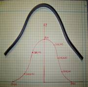
In a previous post (click on the link on the left to learn fully about the experiment, and the assigned problems), I talked

about an experiment we conduct in class to compare spline and polynomial interpolation.  If you do not want to conduct the experiment itself but want the (x,y) data to see for yourself how polynomial and spline interpolation compare, the data is given below.

Length of graduated flexible curve = 12″

The points on the x-y graph are as follows

(-4.1,0), (-2.6,1), (-2.0,2,2), (-1.6, 3.0), (-1,3.6), (0,3.9), (1.6,2.8), (3.2,0.4), (4.1,0)

________________________________________________________________________________________________

This post is brought to you by Holistic Numerical Methods: Numerical Methods for the STEM undergraduate at http://nm.mathforcollege.com.

An abridged (for low cost) book on Numerical Methods with Applications will be in print (includes problem sets, TOC, index) on December 10, 2008 and available at lulu storefront.

Subscribe to the blog via a reader or email to stay updated with this blog. Let the information follow you.

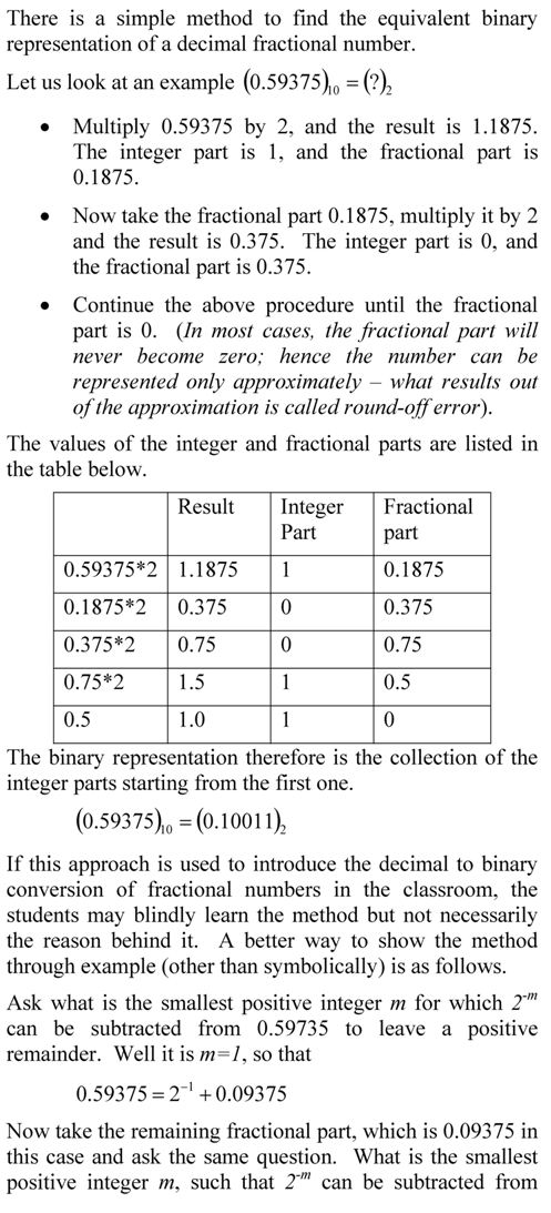
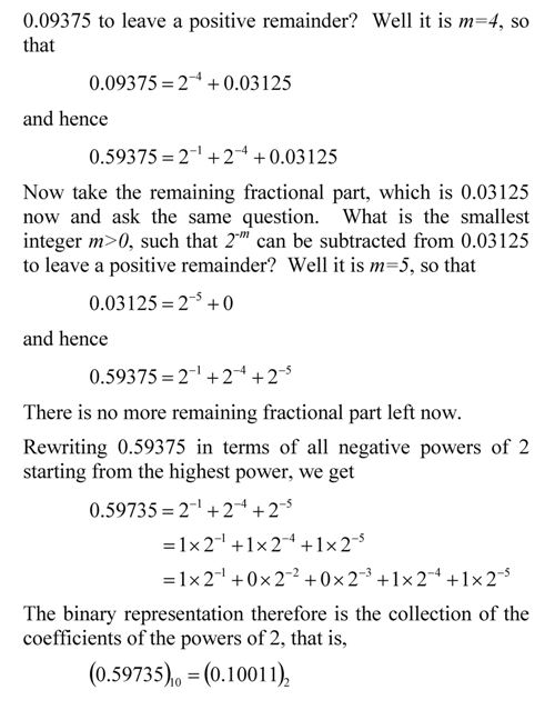
A better way to show conversion of decimal fractional number to binary

This post is brought to you by Holistic Numerical Methods: Numerical Methods for the STEM undergraduate at http://nm.mathforcollege.com, the textbook on Numerical Methods with Applications available from the lulu storefront, and the YouTube video lectures available at http://www.youtube.com/numericalmethodsguy.  

Subscribe to the blog via a reader or email to stay updated with this blog. Let the information follow you.

Finding height of atmosphere using nonlinear regression

Here is an example of finding the height of the atmosphere using nonlinear regression of the mass density of air vs altitude above sea level.

This post is brought to you by Holistic Numerical Methods: Numerical Methods for the STEM undergraduate at http://nm.mathforcollege.com.

An abridged (for low cost) book on Numerical Methods with Applications will be in print (includes problem sets, TOC, index) on December 10, 2008 and available at lulu storefront.

Subscribe to the blog via a reader or email to stay updated with this blog. Let the information follow you.

A better way to show decimal to binary conversion

Decimal to binary conversion of an integer

This post is brought to you by Holistic Numerical Methods: Numerical Methods for the STEM undergraduate at http://nm.mathforcollege.com.

An abridged (for low cost) book on Numerical Methods with Applications will be in print (includes problem sets, TOC, index) on December 10, 2008 and available at lulu storefront.

Subscribe to the blog via a reader or email to stay updated with this blog. Let the information follow you.

Accuracy of Taylor series

So how many terms should I use in getting a certain pre-determined accuracy in a Taylor series. One way is to use the formula for the Taylor’s theorem remainder and its bounds to calculate the number of terms. This is shown in the example below.

Taykor series accuracy

This post is brought to you by Holistic Numerical Methods: Numerical Methods for the STEM undergraduate at http://nm.mathforcollege.com.

An abridged (for low cost) book on Numerical Methods with Applications will be in print (includes problem sets, TOC, index) on December 10, 2008 and available at lulu storefront.

Subscribe to the blog via a reader or email to stay updated with this blog. Let the information follow you.

Taylor series example

If Archimedes were to quote Taylor’s theorem, he would have said, “Give me the value of the function  and the value of all (first, second, and so on) its derivatives at a single point, and I can give you the value of the function at any other point”.

It is very important to note that the Taylor’s theorem is not asking for the expression of the function and its derivatives, just the value of the function and its derivatives at a single point.

Now the fine print: Yes, all the derivatives have to exist and be continuous between x and x+h, the point where you are wanting to calculate the function at. However, if you want to calculate the function approximately by using the nth order Taylor polynomial, then 1st, 2nd,…., nth derivatives need to exist and be continuous in the closed interval [x,x+h], while the (n+1)th derivative needs to exist and be continuous in the open interval (x,x+h).

Taylor Series Revisited

Taylor series is a very important concept that is used in numerical methods. From the concept of truncation error to finding the true error in Trapezoidal rule, having a clear understanding of Taylor series is extremely important. Other places in numerical methods where Taylor series concept is used include: the derivation of finite difference formulas for derivatives, finite difference method of solving differential equations, error in Newton Raphson method of solving nonlinear equations, Newton divided difference polynomial for interpolation, etc.

I have written a short chapter on Taylor series. After reading the chapter, you should be able to:

1. understand the basics of Taylor’s theorem,

2. see how transcendental and trigonometric functions can be written as Taylor’s polynomial,

3. use Taylor’s theorem to find the values of a function at any point, given the values of the function and all its derivatives at a particular point,

4. errors and error bounds of approximating a function by Taylor series,

5. revisit the chapter whenever Taylor’s theorem is used to derive or explain numerical methods for various mathematical procedures.

This post is brought to you by Holistic Numerical Methods: Numerical Methods for the STEM undergraduate at http://nm.mathforcollege.com.

An abridged (for low cost) book on Numerical Methods with Applications will be in print (includes problem sets, TOC, index) on December 10, 2008 and available at lulu storefront.

Subscribe to the blog via a reader or email to stay updated with this blog. Let the information follow you.