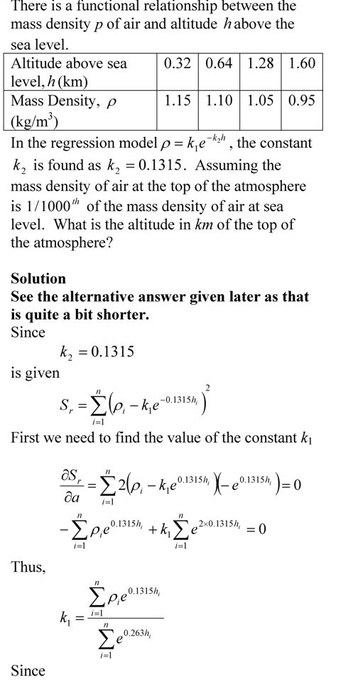
Is it just a coincidence – true error in multiple segment Trapezoidal rule gets approximately quartered as the number of segments is doubled?

Look at the table below. This is a table that shows the approximate value of the integral

$latex \int_{8}^{30} 2000 ln \frac{140000}{140000-2100t}-9.8t dt $

as a function of the number of segments used in the Trapezoidal rule and the corresponding true error.

n

Value

Et

1

11868

-807

2

11266

-205

3

11153

-91.4

4

11113

-51.5

5

11094

-33.0

6

11084

-22.9

7

11078

-16.8

8

11074

-12.9

The true error for n=1 is -807 and for n=2 is -205. As you can see the quarter of -807 is approximately -201.75 and close to the true error for n=2. Is this a coincidence?

Look at the true error for n=2 which is -205 and for n=4 is -51.5. As you can see the quarter of -205 is approximately -51.75 and close to the value of the true error for n=4. Is this a coincidence?

No. This is because the true error in a single segment trapezoidal rule is

$latex \frac{(b-a)^3}{12} f^{\prime\prime} (c)$

where c is some point not known but in the domain [a,b] of $latex \int_{a}^{b} f(x) dx$. It can be then shown (see page 14 of this pdf file for full proof) that for the multiple segment trapezoidal rule, the true error is

$latex \frac{(b-a)^3}{12n^2} f^{\prime\prime} $

where the $latex f^{\prime\prime}$ is an average value of the second derivative of the function f(x) calculated at some point within each of the n segments. Since a and b are constant, and $latex f^{\prime\prime}$ becomes almost a constant as n increases, the true error is approximately inversely proportional to the square of the number of segments.

Note to the reader: Develop a similar table as given above for an integral of your choice and see it for yourself if the true error gets approximately quartered as the number of segments is doubled.

_____________________________________________________

This post is brought to you by Holistic Numerical Methods: Numerical Methods for the STEM undergraduate at http://nm.mathforcollege.com

Subscribe to the blog via a reader or email to stay updated with this blog. Let the information follow you.

Can I use Trapezoidal rule to calculate an improper integral?

For example, $latex \int_{a}^{infinity} e^{-x} dx $ is an improper integral which can be calculated exactly as $latex e^{-a}$.

Can we solve this integral by multiple segment Trapezoidal rule when we already know that the upper limit is infinity?

Yes, we can solve it in spite of the upper limit being infinity. We first need to make a change of variables such as $latex t=\frac{1}{x}$, then $latex dx=-\frac{1}{t^2}dt$ giving $latex \int_{1/a}^{0} e^{-1/t} (-1/t^2) dt $

But even for this integral we have issues as the integrand gives division by zero problems at t=0 (although the limit itself is zero at t=0).

The MATLAB program that can be downloaded at http://nm.mathforcollege.com/blog/trapezoidal_improper.m (better to download it as the single quotes do not translate well with matlab editor) shows that we get accurate results for transformed integral with 256 segments.
% Simulation : Can I use Trapezoidal rule for an improper integral?
% Language : Matlab 2007a
% Authors : Autar Kaw, http://nm.mathforcollege.com
% mfile available at
% http://nm.mathforcollege.com/blog/trapezoidal_improper.m
% Last Revised : July 15, 2008
% Abstract: This program shows use of multiple segment Trapezoidal
% rule to integrate exp(-x) from x=a to infinity, where a>0.
clc
clear all
disp(‘This program shows the convergence of getting the value of ‘)
disp(‘an improper integral using multiple segment Trapezoidal rule’)
disp(‘Author: Autar K Kaw. autarkaw.wordpress.com’)

%INPUTS. If you want to experiment, these are the only variables
% you should and can change.
% a = Lower limit of integration
a=1/2;

fprintf(‘\nFinding the integral of exp(-x) from a to infinity where a=%g’,a)

% SIMULATION
syms x
% integrand exp(-x)
f=exp(-x);
valexact=double(int(f,x,a,inf));
fprintf(‘\n\nExact value of integral = %f’,valexact)
disp( ‘ ‘)

% Transformed integrand by change of variables
ft=inline(‘exp(-1/t)*(-1/t^2)’);
% Limits of integration
at=1/a;
b=0;

%finding value of the integral using 16, 32, 64, 128 and 256 segments
for k=4:1:8
n=2^k;
h=(b-at)/n;
sum=0;
for i=1:1:n-1
sum=sum+ft(at+i*h);
end
% See how f(b) is not added as f(b)=infinity. But
% using a different value of the function at one point or
% finite number of points does not change the value of the
% integral. We are substituting f(b)=0
sum=2*sum+ft(at)+0;
sum=(b-at)/(2*n)*sum;
fprintf(‘\nApproximate value of integral =%f with %g segments’,sum,n)
end
disp(‘ ‘)
This program shows the convergence of getting the value of
an improper integral using multiple segment Trapezoidal rule
Author: Autar K Kaw. autarkaw.wordpress.com

Finding the integral of exp(-x) from a to infinity where a=0.5

Exact value of integral = 0.606531

Approximate value of integral =0.605971 with 16 segments
Approximate value of integral =0.606496 with 32 segments
Approximate value of integral =0.606521 with 64 segments
Approximate value of integral =0.606528 with 128 segments
Approximate value of integral =0.606530 with 256 segments

Published with MATLAB® 7.3

Now someone may rightly point out that it works well because the limit of the integrand is zero at the lower limit of integration for the above mentioned integral.

So go ahead, modify the program for doing this improper integral $latex \int_{0}^{4} \frac{1}{\sqrt {x}} dx $ and see how well it works. In this case the integrand is singular at $latex x=0$ and one would have to assume the function to be a number other than infinity at $latex x=0$ for applying the multiple segment Trapezoidal rule.

How many segments do you need to get an accurate answer for this integral?

_____________________________________________________

This post is brought to you by Holistic Numerical Methods: Numerical Methods for the STEM undergraduate at http://nm.mathforcollege.com

Subscribe to the blog via a reader or email to stay updated with this blog. Let the information follow you.

A metric for measuring wildness of a college football season

A Metric to Quantify the Topsy-Turvyness (Wildness) of a College Football Season

The 2008 college football season is almost here, and news media, sports commentators, and bloggers will hope for something to hype about. Luckily for them, the 2007 season did give them something to talk about; you would be hard pressed to recall a more topsy-turvy season. Ranked teams regularly lost to low-ranked and unranked teams.

In just Week#1 of the 2007 season, Associated Press (AP) No. 5 team University of Michigan lost to an unranked Division II team – Appalachian State. The Associated Press wasted no time in booting out Michigan out of the Top AP 25. Two weeks later, No. 11 UCLA lost to unranked Utah by a wide margin of 44-6. UCLA also met the same fate as Michigan; UCLA was dropped from the AP Top 25.

The topsy-turvyness continued in the season, especially for No. 2 ranked teams. The University of South Florida, where I work, was ranked No. 2 when they lost to unranked Rutgers 30-27 in Week#8. This was the same week when three other teams (South Carolina, Kentucky, and California) ranked in the Top 10 of the AP poll also lost their games.

To top off the season, for the first time in history of the Bowl Championship Series (BCS), the title bowl game had a team (Louisiana State University (LSU)) with two regular season losses, and LSU ended up winning the national championship.

Although many ranted and raved about the anecdotal evidence of a topsy-turvy season, is it possible that the media and fans over exaggerated the topsy-turvyness of the 2007 college football season. Were there other seasons that were more topsy-turvy than 2007?

To answer this question scientifically, this article proposes an algorithm to quantify the topsy-turvyness of the college football season. The author does not know of any previous literature that has attempted to develop a metric that quantifies the topsy-turvyness of any sport, which is ranked regularly in the season.

The TT factor

The Topsy-Turvy Factor (TT factor) is a metric that quantifies the topsy-turvyness of a college football season. Two different TT factors are calculated: one for each of week of the season, referred to as the Week TT factor, and one for the cumulative topsy-turvyness at the end of each week of the season, referred to as the Season TT factor.

The method to find the Week TT Factor is based on comparing the AP Top 25 poll rankings of schools from the current week to that of the previous week. The difference in the rankings of each school in the AP Top 25 from the current week to the previous week is squared. How do we account for teams that fall out of the rankings? A team that gets unranked from the previous week is assumed as having become the No. 26 team in the current week. All the squares of the differences in the rankings are then added together and normalized on a scale of 0-100.

The other TT factor, the Season TT factor is also calculated for the end of each week to gage how topsy-turvy the season has been so far. The Season TT factor is calculated using weighted averages of the Week TT factors. As the season progresses, the Week TT factors are given more weight in the calculation of the Season TT factor because toward the end of the season, an upset of a ranked team is more topsy-turvy than an upset in the beginning of the season when the strength of a ranked team is less established.

Season End of Season TT factor
2007 ……………..60
2006 ……………..46
2005 ……………..48
2004 ……………..40
2003 ……………. 55
2002 ……………. 48

Table 1: End of Season TT factors for 2002-2007 Seasons

Table 1 shows the end of Season TT factor of the last six football seasons. It is clear that 2007 was the most topsy-turvy season in recent history, with the 2003 season not too far behind. In contrast, the 2004 season was the least topsy-turvy.

Read the complete paper including formulas and detailed analysis at

http://www.eng.usf.edu/~kaw/TT_factor_paper_media.pdf

Can you write a program in MATLAB or any other language to find the Week TT factors and the Season TT factors?

_____________________________________________________

This post is brought to you by Holistic Numerical Methods: Numerical Methods for the STEM undergraduate at http://nm.mathforcollege.com

Subscribe to the blog via a reader or email to stay updated with this blog. Let the information follow you.

Experiment for spline interpolation and integration

Background:

The motivation behind the experiment is to understand spline interpolation and numerical integration by finding the volume of water that can be held by a champagne glass.

What does the student do in the lab:

The student chooses one of the odd-shaped champagne glasses (Figure 1). The student measures the outer radius of the champagne glass at different known locations along the height. The student measures the thickness of the glass, so that he/she will be able to find the inner radius of the champagne glass at the locations he/she measured the outer radius. The student pours water to the brim in the champagne glass and checks how much volume the champagne glass holds.

Champagne GlassExercises assigned to the students:
Use MATLAB to solve problems. Use comments, display commands and fprintf statements, sensible variable names and units to explain your work. Staple all the work in the following sequence. Use USCS system of units throughout.

  1. Attach the data sheet on which you collected the data in class.
  2. Find the spline interpolant that curve fits the radius vs height data.
  3. Show the individual points and the spline interpolant of radius vs height on a single plot.
  4. Find how much volume of water the champagne glass would hold.
  5. Compare the above result from problem#4 to the actual volume.
  6. In 100-200 words, type out your conclusions using a word processor. Any formulas should be shown using an equation editor. Any sketches need to be drawn using a drawing software such as Word Drawing. Any plots can be imported from MATLAB.

What materials do you need; where do I buy it; how much do the materials costs?

  1. Champagne Glasses: These glasses, called the Hurricane Plastic Glasses, are available at www.poolsidepineapple.com, part nos. HUR-105, HUR-106, YAR-114. We used glasses made of plastic to avoid breakage. http:/www.poolsidepineapple.com/cart_pages/shopping%20page%20tropical.htm. You can try other places to buy the champagne glasses. About $40 or so for about six pieces including S&H. Better yet, go to a cruise and get souvenir glasses. Whenever you do the experiment, you will remember the good times.
  2. Graduated Cylinder: The graduated cylinder is available at http://scientificsonline.com/, part number 3036286. The cost of the cylinder is $20+S&H.
  3. Vernier Caliper: The caliper is available at http://mcmaster.com part number 20265A49. The cost of the vernier caliper is $60+S&H.
  4. Scale: Need to buy a thin scale for this. Any art-supplies store for $2 or so.

_____________________________________________________

This post is brought to you by Holistic Numerical Methods: Numerical Methods for the STEM undergraduate at http://nm.mathforcollege.com

Subscribe to the blog via a reader or email to stay updated with this blog. Let the information follow you.

Abuses of regression

There are three common abuses of regression analysis.

  1. Extrapolation
  2. Generalization
  3. Causation.

Extrapolation

If you were dealing in the stock market or even interested in it, we remember the stock market crash of March 2000. During 1997-1999, many investors thought they would double their money every year, started buying fancy cars and houses on credit, and living the high life. Little did they know that the whole market was hyped on speculation and little economic sense? Enron and MCI financial fiascos were soon to follow.

Let us look if we could have safely extrapolated NASDAQ index from past years. Below is the table of NASDAQ index, S as a function of end of year number, t (Year 1 is the end of year 1994, and Year 6 is the end of year 1999).

Table 1 NASDAQ index as a function of year number.

Year Number (t)

NASDAQ Index (S)

1 (1994)

752

2 (1995)

1052

3 (1996)

1291

4 (1997)

1570

5 (1998)

2193

6 (1999)

4069

A relationship S = a0+a1t+a2t2 between the NASDAQ index, S and the year number, t is developed using least square regression and is found to be

S=168.14t2 – 597.35t + 1361.8

The data is given for Years 1 thru 6 and it is desired to calculate the value for t>=6. This is extrapolation outside the model data. The error inherent in this model is shown in Table 2. Look at the Year 7 and 8 that was not included in the regression data – the error between the predicted and actual values is 119% and 277%, respectively.

 Table 2 NASDAQ index as a function of year number.

Year Number

(t)

NASDAQ Index

(S)

Predicted Index

Absolute Relative True Error (%)

1 (1994)

752

933

24

2 (1995)

1052

840

20

3 (1996)

1291

1082

16

4 (1997)

1570

1663

6

5 (1998)

2193

2578

18

6 (1999)

4069

3831

6

7 (2000)

2471

5419

119

8 (2001)

1951

7344

277

This illustration is not exaggerated and it is important that a careful use of any given model equations is always called for. At all times, it is imperative to infer the domain of independent variables for which a given equation is valid.


Generalization

Generalization could arise when unsupported or overexaggerated claims are made. It is not often possible to measure all predictor variables relevant in a study. For example, a study carried out about the behavior of men might have inadvertently restricted the survey to Caucasian men. Shall we then generalize the result as the attributes of all men irrespective of race? Such use of regression equation is an abuse since the limitations imposed by the data restrict the use of the prediction equations to Caucasian men.


Misidentification

Finally, misidentification of causation is a classic abuse of regression analysis equations. Regression analysis can only aid in the confirmation or refutation of a causal model ‑ the model must however have a theoretical basis. In a chemical reacting system in which two species react to form a product, the amount of product formed or amount of reacting species vary with time. Although a regression equation of species concentration and time can be obtained, one cannot attribute time as the causal agent for the varying species concentration. Regression analysis cannot prove causality; rather they can only substantiate or contradict causal assumptions. Anything outside this is an abuse of the use of regression analysis method.

This post used textbook notes written by the author and Egwu Kalu, Professor of Chemical and Biomedical Engineering, FAMU, Tallahassee, FL.

____________________________________________________

This post is brought to you by Holistic Numerical Methods: Numerical Methods for the STEM undergraduate at http://nm.mathforcollege.com

Subscribe to the blog via a reader or email to stay updated with this blog. Let the information follow you.


How do you know that the least squares regression line is unique and corresponds to a minimum

We already know that using the criterion of either

  1. minimizing sum of residuals OR
  2. minimizing sum of the absolute value of residuals

is BAD as either of the criteria do not give a unique line. Visit these notes for an example where these criteria are shown to be inadequate.

So we use minimizing the sum of the squares of the residuals as the criterion. How can we show that this criterion gives a unique line?

The proof is given below as image files because the proof is equation intensive. I made a better resolution pdf file also.


_____________________________________________________

This post is brought to you by Holistic Numerical Methods: Numerical Methods for the STEM undergraduate at http://nm.mathforcollege.com

Subscribe to the blog via a reader or email to stay updated with this blog. Let the information follow you.

Finding the optimum polynomial order to use for regression

Many a times, you may not have the privilege or knowledge of the physics of the problem to dictate the type of regression model. You may want to fit the data to a polynomial. But then how do you choose what order of polynomial to use.

Do you choose based on the polynomial order for which the sum of the squares of the residuals, Sr is a minimum? If that were the case, we can always get Sr=0 if the polynomial order chosen is one less than the number of data points. In fact, it would be an exact match.

So what do we do? We choose the degree of polynomial for which the variance as computed by

Sr(m)/(n-m-1)

is a minimum or when there is no significant decrease in its value as the degree of polynomial is increased. In the above formula,

Sr(m) = sum of the square of the residuals for the mth order polynomial

n= number of data points

m=order of polynomial (so m+1 is the number of constants of the model)

Let’s look at an example where the coefficient of thermal expansion is given for a typical steel as a function of temperature. We want to relate the two using polynomial regression.

Temperature

Instantaneous Thermal Expansion

oF

1E-06 in/(in oF)

80

6.47

40

6.24

0

6.00

-40

5.72

-80

5.43

-120

5.09

-160

4.72

-200

4.30

-240

3.83

-280

3.33

-320

2.76

If a first order polynomial is chosen, we get

$latex alpha=0.009147T+5.999$, with Sr=0.3138.

If a second order polynomial is chosen, we get

$latex alpha=-0.00001189T^2+0.006292T+6.015$ with Sr=0.003047.

Below is the table for the order of polynomial, the Sr value and the variance value, Sr(m)/(n-m-1)

Order of

polynomial, m

Sr(m)

Sr(m)/(n-m-1)

1

0.3138

0.03486

2

0.003047

0.0003808

3

0.0001916

0.000027371

4

0.0001566

0.0000261

5

0.0001541

0.00003082

6

0.0001300

0.000325

So what order of polynomial would you choose?

From the above table, and the figure below, it looks like the second or third order polynomial would be a good choice as very little change is taking place in the value of the variance after m=2.

Optimum order of polynomial for regression

This post is brought to you by Holistic Numerical Methods: Numerical Methods for the STEM undergraduate at http://nm.mathforcollege.com

Subscribe to the feed to stay updated and let the information follow you.

Data for aluminum cylinder in iced water experiment

A colleague asked me what if he did not have time or resources to do the experiments that have been developed at University of South Florida (USF) for numerical methods. He asked if I could share the data taken at USF.

Why not – here is the data for the experiment where an aluminum cylinder is placed in iced water. This link also has the exercises that the students were asked to do.

The temperature vs time data is as follows: (0,23.3), (5,16.3), (10,13), (15,11.8), (20,11), (25,10.7), (30,9.6), (35,8.9), (40,8.4). Time is in seconds and temperature in Celcius. Other data needed is

Ambient temperature of iced water = 1.1oC

Diameter of cylinder = 44.57 mm

Length of cylinder = 105.47 mm

Density of aluminum = 2700 kg/m3

Specific heat of aluminum = 901 J/(kg-oC)

Thermal conductivity of aluminum = 240 W/(m-K)

Table 1. Coefficient of thermal expansion vs. temperature for aluminum (Data taken from http://www.llnl.gov/tid/lof/documents/pdf/322526.pdf by using mid values of temperatures at which CTE is reported)

Temperature

(oC)

Coefficient of thermal expansion

(μm/m/oC)

-10

58

12.5

59

37.5

60

62.5

62

87.5

66

112.5

71

This post is brought to you by Holistic Numerical Methods: Numerical Methods for the STEM undergraduate at http://nm.mathforcollege.com

Subscribe to the feed to stay updated and let the information follow you.

In regression, when is coefficient of determination zero

The coefficient of determination is a measure of how much of the original uncertainty in the data is explained by the regression model.

The coefficient of determination, $latex r^2$ is defined as

$latex r^2$=$latex \frac{S_t-S_r}{S_r}$

where

$latex S_t$ = sum of the square of the differences between the y values and the average value of y

$latex S_r$ = sum of the square of the residuals, the residual being the difference between the observed and predicted values from the regression curve.

The coefficient of determination varies between 0 and 1. The value of the coefficient of determination of zero means that no benefit is gained by doing regression. When can that be?

One case comes to mind right away – what if you have only one data point. For example, if I have only one student in my class and the class average is 80, I know just from the average of the class that the student’s score is 80. By regressing student score to the number of hours studied or to his GPA or to his gender would not be of any benefit. In this case, the value of the coefficient of determination is zero.

What if we have more than one data point? Is it possible to get the coefficient of determination to be zero?

The answer is yes. Look at the following data pairs (1,3), (3,-2), (5,4), (7,-5), (9,4.2), (11,3), (2,4). If one regresses this data to a general straight line

y=a+bx,

one gets the regression line to be

y=1.6

When is rsquared zero?

In fact, 1.6 is the average value of the given y values. Is this a coincidence? Because the regression line is the average of the y values, $latex S_t=S_r$, implying $latex r^2=0$

QUESTIONS

  1. Given (1,3), (3,-2), (5,4), (7,a), (9,4.2), find the value of a that gives the coefficient of determination, $latex r^2=0$. Hint: Write the expression for $latex S_r$ for the regression line $latex y=mx+c$. We now have three unknowns, m, c and a. The three equations then are $latex \frac{\partial S_r} {\partial m} =0$, $latex \frac{\partial S_r} {\partial c} =0$ and $latex S_t=S_r$.
  2. Show that if n data pairs $latex (x_1,y_1)……(x_n,y_n)$ are regressed to a straight line, and the regression straight line turns out to be a constant line, then the equation of the constant line is always y=average value of the y-values.

This post is brought to you by Holistic Numerical Methods: Numerical Methods for the STEM undergraduate at http://nm.mathforcollege.com

Subscribe to the feed to stay updated and let the information follow you.

Length of a curve experiment

In a previous post, I mentioned that I have incorporated experiments in my Numerical Methods course. Here I will discuss the second experiment.

Length of the curve experimentIn this experiment, we find the length of two curves generated from the same points – one curve is a polynomial interpolant and another one is a spline interpolant.

Motivation behind the experiment: In 1901, Runge conducted a numerical experiment to show that higher order interpolation is a bad idea. It was shown that as you use higher order interpolants to approximate f(x)=1/(1+25x2) in [-1,1], the differences between the original function and the interpolants becomes worse. This concept also becomes the basis why we use splines rather than polynomial interpolation to find smooth paths to travel through several discrete points.

What do students do in the lab: A flexible curve (see Figure) of length 12″ made of lead-core construction with graduations in both millimeters and inches is provided. The student needs to draw a curve similar in shape to the Runge’s curve on the provided graphing paper as shown. It just needs to be similar in shape – the student can make the x-domain shorter and the maximum y-value larger or vice-versa. The student just needs to make sure that there is a one-to-one correspondence of values.

Assigned Exercises: Use MATLAB to solve problems (3 thru 6). Use comments, display commands and fprintf statements, sensible variable names and units to explain your work. Staple all the work in the following sequence.

  1. Signed typed affidavit sheet.
  2. Attach the plot you drew in the class. Choose several points (at least nine – do not need to be symmetric) along the curve, including the end points. Write out the co-ordinates on the graphing paper curve as shown in the figure.
  3. Find the polynomial interpolant that curve fits the data. Output the coefficients of the polynomial.
  4. Find the cubic spline interpolant that curve fits the data. Just show the work in the mfile.
  5. Illustrate and show the individual points, polynomial and cubic spline interpolants on a single plot.
  6. Find the length of the two interpolants – the polynomial and the spline interpolant. Calculate the relative difference between the length of each interpolant and the actual length of the flexible curve.
  7. In 100-200 words, type out your conclusions using a word processor. Any formulas should be shown using an equation editor. Any sketches need to be drawn using a drawing software such as Word Drawing. Any plots can be imported from MATLAB.

Where to buy the items for the experiment:

  1. Flexible curves – I bought these via internet at Art City. The brand name is Alvin Tru-Flex Graduated Flexible Curves. Prices range from $5 to $12. Shipping and handling is extra – approximately $6 plus 6% of the price. You may want to buy several 12″ and 16″ flexible curves. I had to send a query to the vendor when I did not receive them within a couple of weeks. Alternatively, call your local Art Store and see if they have them.
  2. Engineering Graph Paper – Staples or Office Depot. Costs about $12 for a pack for 100-sheet pad.
  3. Pencil – Anywhere – My favorite store is the 24-hour Wal-Mart Superstore. $1 for a dozen.
  4. Scale – Anywhere – My favorite store is the 24-hour Wal-Mart Superstore. $1 per unit.

This post is brought to you by Holistic Numerical Methods: Numerical Methods for the STEM undergraduate at http://nm.mathforcollege.com

Subscribe to the feed to stay updated and let the information follow you.