How do I do that in MATLAB

HOW DO I DO THAT IN MATLAB SERIES?

How do I solve simultaneous linear equations given in equation form? Updated Matlab 2018b

Guest co-blogger: : Luis Serrano

Many students ask me how do I do this or that in MATLAB.  So I thought why not have a small series of my next few blogs do that.  In this blog, I show you how to solve simultaneous linear equations given in equation form.

  • The MATLAB program link is here.
  • The HTML version of the MATLAB program is here.
  • DO NOT COPY AND PASTE THE PROGRAM BELOW BECAUSE THE SINGLE QUOTES DO NOT TRANSLATE TO THE CORRECT SINGLE QUOTES IN MATLAB EDITOR.  DOWNLOAD THE MATLAB PROGRAM INSTEAD

%% SUMMARY
% Language : Matlab 2018b;
% Authors : Autar Kaw and Luis Serrano;
% Mfile available at
% http://nm.mathforcollege.com/blog/SimultaneousEquationsEqForm.m;
% Last Revised : January 22, 2020;
% Abstract: This program shows you how to solve a set of
% simultaneous linear equations given in equation form?
% .
clc
clear all
%% INTRODUCTION
disp(‘ABSTRACT’)
disp(‘ This program shows you how to solve a’)
disp(‘ set of simultaneous linear equations given in equation form’)
disp(‘ ‘)
disp(‘AUTHOR’)
disp(‘ Autar Kaw and Luis Serrano’)
disp(‘ ‘)
disp(‘MFILE SOURCE’)
disp(‘ http://nm.mathforcollege.com/blog/SimultaneousEquationsEqForm.m’)
disp(‘ ‘)
disp(‘LAST REVISED’)
disp(‘ January 22, 2020’)
disp(‘ ‘)
%% INPUTS
% Enter the equations
syms a b c
eqn1=12*a+23*b+39*c==29
eqn2=13*a+17*b+19*c==37
eqn3=21*a+23*b+29*c==59
%% DISPLAYING INPUTS
disp(‘ ‘)
disp(‘INPUTS’)
disp(‘________________________’)
disp(‘Equations’)
disp(‘________________________’)
disp(eqn1)
disp(eqn2)
disp(eqn3)
%% THE CODE
% The solution
X=solve(eqn1,eqn2,eqn3);
% Assigning the output
a=double(X.a);
b=double(X.b);
c=double(X.c);
%% DISPLAYING OUTPUTS
disp(‘ ‘)
disp(‘OUTPUTS’)
disp(‘________________________’)
disp(‘Solution Vector’)
disp(‘________________________’)
fprintf(‘\nValue of a= %g’,a)
fprintf(‘\nValue of b= %g’,b)
fprintf(‘\nValue of c= %g’,c)
disp(‘ ‘)
disp(‘________________________’)

_______________________

This post is brought to you by

The program to find the determinant of matrix

Here is the MATLAB program to find the determinant of a nxn matrix by the cofactor method.  I had to develop a separate function for each size of the matrix.  I may be wrong about having to do that – is there a single function that can be written to find the determinant of any nxn matrix using the cofactor method?

The mfile can be downloaded here.   Try the program for a 10×10 matrix – it took about 6 seconds of CPU time on my PC.  A 12×12 matrix determinant would take about 13 minutes of CPU time.  I stopped at a 12×12 matrix.  You can either write a function or generate the function via a program for matrices of 13×13 order and higher.

Contents

Finding the determinant of a matrix using the cofactor method

and comparing the CPU time with MATLAB det function

clc
clear all
format long

% n=Size of matrix
n=6;
% Choosing a matrix of nxn size with random numbers
A=rand(n,n);

% Calculating cputime by cofactor method
tbegin=cputime;
detval=det6(A);
TimeCrammer=cputime-tbegin;

% Calculating cputime by MATLAB det function
tbegin=cputime;
MatlabDet=det(A);
TimeMatlab=vpa(cputime-tbegin,32);

% Printing the times
fprintf('Size of matrix is %gx%g \n',n,n)
fprintf('Determinant by cofactor method = %g \n', detval)
fprintf('Determinant by Matlab function = %g \n', MatlabDet)
fprintf('Approximate CPU time taken by cofactor method = %g seconds\n',TimeCrammer)
fprintf('Approximate CPU time taken by MATLAB function = %e seconds\n',TimeMatlab)

Individual functions for determinant of a nxn matrix

function detvalue=det2(A)
detvalue=A(1,1)*A(2,2)-A(1,2)*A(2,1);
end

function detvalue=det3(A)
n=3;
detvalue=0;
for j=1:1:n
    detvalue=detvalue+(-1)^(j+1)*A(1,j)*det2(A(2:n,[1:j-1 j+1:n]));
end
end

function detvalue=det4(A)
n=4;
detvalue=0;
for j=1:1:n
    detvalue=detvalue+(-1)^(j+1)*A(1,j)*det3(A(2:n,[1:j-1 j+1:n]));
end
end

function detvalue=det5(A)
n=5;
detvalue=0;
for j=1:1:n
    detvalue=detvalue+(-1)^(j+1)*A(1,j)*det4(A(2:n,[1:j-1 j+1:n]));
end
end

function detvalue=det6(A)
n=6;
detvalue=0;
for j=1:1:n
    detvalue=detvalue+(-1)^(j+1)*A(1,j)*det5(A(2:n,[1:j-1 j+1:n]));
end
end

function detvalue=det7(A)
n=7;
detvalue=0;
for j=1:1:n
    detvalue=detvalue+(-1)^(j+1)*A(1,j)*det6(A(2:n,[1:j-1 j+1:n]));
end
end
function detvalue=det8(A)
n=8;
detvalue=0;
for j=1:1:n
    detvalue=detvalue+(-1)^(j+1)*A(1,j)*det7(A(2:n,[1:j-1 j+1:n]));
end
end

function detvalue=det9(A)
n=9;
detvalue=0;
for j=1:1:n
    detvalue=detvalue+(-1)^(j+1)*A(1,j)*det8(A(2:n,[1:j-1 j+1:n]));
end
end

function detvalue=det10(A)
n=10;
detvalue=0;
for j=1:1:n
    detvalue=detvalue+(-1)^(j+1)*A(1,j)*det9(A(2:n,[1:j-1 j+1:n]));
end
end

function detvalue=det11(A)
n=11;
detvalue=0;
for j=1:1:n
    detvalue=detvalue+(-1)^(j+1)*A(1,j)*det10(A(2:n,[1:j-1 j+1:n]));
end
end

function detvalue=det12(A)
n=12;
detvalue=0;
for j=1:1:n
    detvalue=detvalue+(-1)^(j+1)*A(1,j)*det11(A(2:n,[1:j-1 j+1:n]));
end
end
Size of matrix is 6x6 
Determinant by cofactor method = -0.0431 
Determinant by Matlab function = -0.0431 
Approximate CPU time taken by cofactor method = 0.140625 seconds
Approximate CPU time taken by MATLAB function = 1.562500e-02 seconds

The above mfile can be downloaded here.


This post is brought to you by


Time it takes to find a determinant

To make the point of how inefficient it is to find the determinant of a matrix by the cofactor method, I wrote a program in MATLAB to demonstrate this.  A google search for a program written in any language to find the determinant by using the cofactor method was not available beyond a 4×4 matrix.  So, I wrote one that finds the determinant of matrices of up to 12×12 order.

I ran the program on an Intel(R) Core(TM) i5-8500 CPU @3.00GHz PC.  Here is a table of the CPU time it took in seconds to find the determinant of a matrix as a function of its order.
______________________________________
Order of matrix               CPU Time to Find
Determinant (s)
______________________________________
6×6                                           0.015625
7×7                                           0.046875
8×8                                           0.203125
9×9                                           0.828125
10×10                                        5.14063
11×11                                       52.6406
12×12                                   623.953
______________________________________

If one continues to do this for a 25×25 matrix, it is estimated that it would take 8.1821198 \times 10^{17} seconds which is more than 25 billion years, and we all know that the estimated age of the universe is less at about 13.77 billion years.

The trend of the approximate time it takes to find the determinant of the next order of the matrix, nxn is approximately n times the time it takes to find the determinant of a (n-1)x(n-1) matrix.  For example, it took a time of 52.6406 seconds for finding the determinant of a 11×11 matrix, while it would be estimated to take approximately 12×52.6406=631.7 seconds for finding the determinant of a 12×12 matrix.  This is close to the 623.953 seconds it actually took.

The above approximate time calculations are in concurrence with the note written by Professor A.J. Wise in 1969, where he showed that the number of arithmetic operations required to evaluate a nxn determinant by cofactor method is given by [n!e]-2, and hence n!e for large n and the time it takes to find the determinant of the next order of the matrix, nxn is approximately n times the time it takes to find the determinant of a (n-1)x(n-1) matrix

Since the arithmetic operation required here are just addition, multiplication and subtraction, the computation time could be crudely estimated as 4Tn!e for large n, where T is the clock cycle time and we assume that an addition or a multiplication or a subtraction each use 4 clock cycle times.  Does it match?

For a 3.00 GHz machine, T={1}/({3 \times 10^9}) seconds to give an approximate time for a 12×12 matrix determinant calculation to be 4 \times {1}/{(3 \times 10^9)} \times 12! e = 1.736  seconds.  It is not even of similar order.  Many items go into calculating CPU time for a numerical algorithm, but to do a comparative analysis, these calculations are quite helpful.


This post is brought to you by

Matrix Algebra: Gauss-Seidel Method

Many university STEM major programs have reduced the credit hours for a course in Matrix Algebra or have simply dropped the course from their curriculum.   The content of Matrix Algebra in many cases is taught just in time where needed.  This approach can leave a student with many conceptual holes in the required knowledge of matrix algebra. In this series of blogs, we bring to you ten topics that are of immediate and intermediate interest for Matrix Algebra. Here is the eighth topic where we talk about solving a set of simultaneous linear equations using the Gauss-Seidel method.  Learn this iterative method of solving simultaneous linear equations, and its pitfalls and advantages. Get all the resources in form of textbook content, lecture videos, multiple choice test, problem set, and PowerPoint presentation. Gauss-Seidel Method
This post is brought to you by

Matrix Algebra: LU Decomposition Method

Many university STEM major programs have reduced the credit hours for a course in Matrix Algebra or have simply dropped the course from their curriculum.   The content of Matrix Algebra in many cases is taught just in time where needed.  This approach can leave a student with many conceptual holes in the required knowledge of matrix algebra. In this series of blogs, we bring to you ten topics that are of immediate and intermediate interest for Matrix Algebra. Here is the seventh topic where we talk about solving a set of simultaneous linear equations using the LU decomposition method.  First, the LU decomposition method is discussed along with its motivation.  The LU decomposition method to find the inverse of a square matrix is discussed. Get all the resources in form of textbook content, lecture videos, multiple choice test, problem set, and PowerPoint presentation. LU Decomposition Method
This post is brought to you by

Computational Time for Forward Elimination Steps of Naive Gaussian Elimination on a Square Matrix

Problem Statement

How much computational time does it take to conduct the forward elimination part of the Naïve Gauss Elimination method on a square matrix?

CTdecomposition

This post is brought to you by

Clearing up the confusion about diagonally dominant matrices – Part 2

In a previous post, we discussed the confusion about the definition and associated properties of diagonally dominant matrices.  In this blog, we answer the next question.

What is a weak diagonally dominant matrix?

The answer is simple – the definition of a weak(ly) diagonally dominant matrix is identical to that of a diagonally dominant matrix as the inequality used for the check is a weak inequality of greater than or equal to (≥).  See the previous post on Clearing up the confusion about diagonally dominant matrices – Part 1 where we define a diagonally dominant matrix.

Other blogs on diagonally dominant matrices
Clearing up the confusion about diagonally dominant matrices – Part 1

_______________________________________

This post is brought to you by


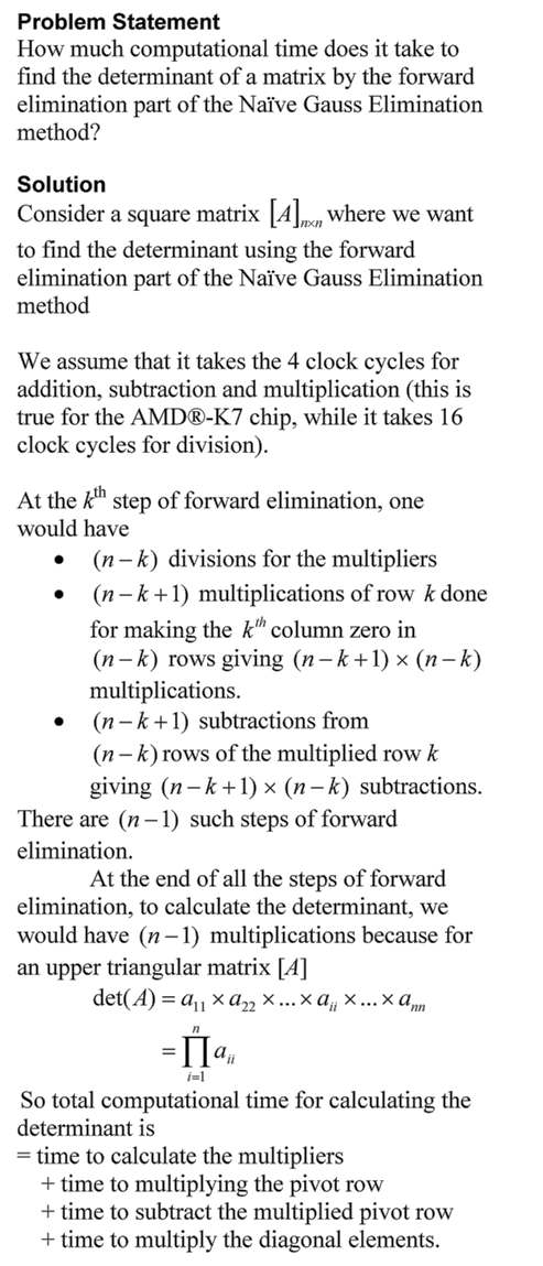
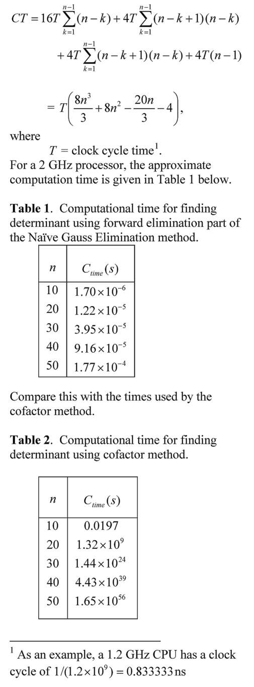
Computational Time to Find Determinant Using Gaussian Elimination

The time it would take to find the determinant of a matrix using the Gaussian Elimination is many-many orders less than when the cofactor method is used.  In this blog, we derive the formula for a typical amount of computational time it would take to find the determinant of a nxn matrix using the forward elimination part of the Naive Gauss Elimination method.  The time is compared with that using the cofactor method.
 Computational time to find determinant

Computational time to find determinant

This post is brought to you by Holistic Numerical Methods: Numerical Methods for the STEM undergraduate at http://nm.mathforcollege.com, the textbook on Numerical Methods with Applications available from the lulu storefront, the textbook on Introduction to Programming Concepts Using MATLAB, and the YouTube video lectures available at http://nm.mathforcollege.com/videos.  Subscribe to the blog via a reader or email to stay updated with this blog. Let the information follow you.

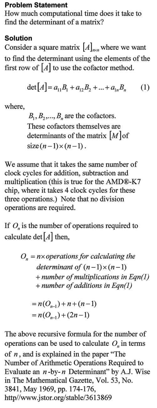
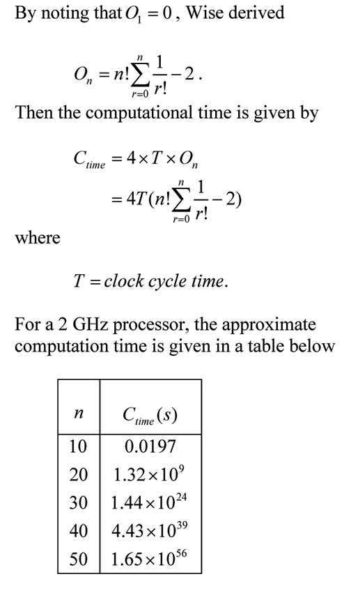
Computational Time to Find Determinant Using CoFactor Method

The time it would take to find the determinant of a matrix using the cofactor method can be daunting.  A student may not realize this as they may be limited to finding determinants of matrices of order 4×4 or less by hand.  In this blog, we derive the formula for a typical amount of computational time it would take to find the determinant of a nxn matrix using the cofactor method.
 Computational time to find determinant

Computational time to find determinant

This post is brought to you by Holistic Numerical Methods: Numerical Methods for the STEM undergraduate at http://nm.mathforcollege.com, the textbook on Numerical Methods with Applications available from the lulu storefront, the textbook on Introduction to Programming Concepts Using MATLAB, and the YouTube video lectures available at http://nm.mathforcollege.com/videos.  Subscribe to the blog via a reader or email to stay updated with this blog. Let the information follow you.